ABSTRACT
In preceding publications, the accuracy of interpolation using reference functions for temperature sensors (thermocouples and platinum resistance thermometers (PRTs)), as well as a crude approach to interpolation uncertainty in the absence of any knowledge of the interpolating function, have been discussed. This article discusses how to fit curves to PRT calibration results using the linear least squares technique (implemented using matrix functions in Microsoft Excel or Libreoffice Calc), both directly to the measured data and to deviations from a reference function. (An overview of the fitting method may be found in [Numerical Recipes in Fortran 77, Chapter 15. Modeling of data].)
INTRODUCTION
In the preceding articles, we saw that
(i) industrial PRT calibration results could be interpolated “piece-wise” (between any two calibration points a few hundred degrees Celsius apart) to an accuracy of around 0.05 °C, when expressed as deviations from the Callendar-van Dusen reference functions, and,
(ii) without any knowledge of the accuracy of the interpolating function, the accuracy of interpolated values could be grossly estimated as 0.15 to 0.5 °C (for the above-mentioned spacing between calibration points).
While the latter approach can be applied generically to almost any calibration data, it has the drawback that the uncertainty of interpolated values is unrealistically large when working close to a calibration point. In the present article, the most accurate approach to the problem will be implemented, namely, to fit a curve to the complete set of calibration results. Firstly, a Callendar equation will be fitted directly to the measured data, and, secondly, a quadratic polynomial will be fitted to the deviations of the measured data from the ITS-90 PRT reference function. As the ITS-90 reference function deals with most PRT non-linearity, it is expected that the latter approach will produce the more accurate interpolation.
THE MODEL EQUATION
The Callendar equation, applicable above 0 °C, is: Rt = R0∙(1 + A∙t + B∙t^2), where Rt is the resistance (in Ω) at temperature t (in °C) and R0 is the resistance (in Ω) at the ice point (0.00 °C). Rearranging the equation, A∙t + B∙t^2 = Rt/R0 – 1, indicating that the independent variable x = t and the dependent variable y = Rt/R0 – 1.
(As the sensitivity. d(Rt/R0)/dt, will be required to convert uncertainties from temperature units, we also note that d(Rt/R0)/dt = A + 2∙B∙t. We will use the coefficients from IEC 60751, namely, A = 3.9083e-3 and B = -5.775e-7, to calculate sensitivities below.)
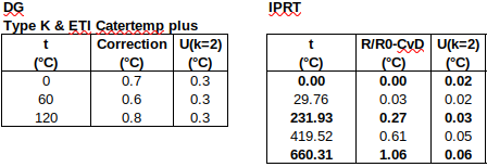
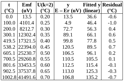
The measured data are as follows:
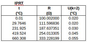
To find R0 from R(0.01 °C): R0 = R(0.01 °C) + (0.00 °C – 0.01 °C) ∙ 0.391 Ω/°C. Uncertainties are converted to the same units as y. (The 1st data point is used to determine R0, so only the four subsequent data points are used in the fit.)

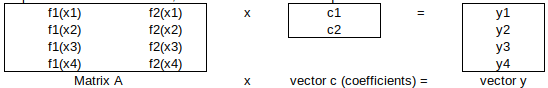
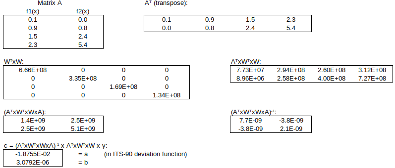
The general model equation is c1∙f1(x) + c2∙f2(x) + … = y. For the Callendar equation, c1 = A, f1(x) = x, c2 = B and f2(x) = x^2.
The four data points lead to four simultaneous equations, namely:
c1∙f1(x1) + c2∙f2(x1) = y1
c1∙f1(x2) + c2∙f2(x2) = y2
c1∙f1(x3) + c2∙f2(x3) = y3
c1∙f1(x4) + c2∙f2(x4) = y4
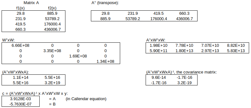
Expressed in matrix notation, they are:
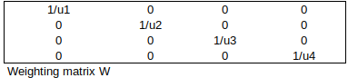
WEIGHTING FACTORS
Now, apply the weighting factors 1/ui to each equation (smaller std uncertainty => larger weight). The weighted simultaneous equations, expressed in matrix notation, are: W x A x c = W x y.
THE SOLUTION – NORMAL EQUATIONS
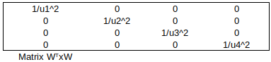
The optimal (least squares) solution to this over-determined system is obtained by left-multiplying by the matrix transpose (WA)T = ATxWT, to obtain the normal equations:
![]()
Matrix WTxW simply contains 1/variance at each calibration point:
![]()
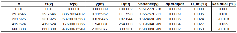
Then, to find the fitted y-value for any value of x:
![]()

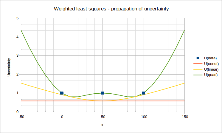
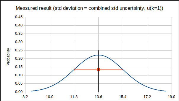
Finally, expanded uncertainty of y = 2*√variance(y): this is called the “propagated uncertainty” of y at x.
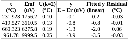
The numerical implementation of this “linear least squares” curve-fitting technique follows, using the Excel or Calc matrix functions TRANSPOSE(), MMULT() and MINVERSE():
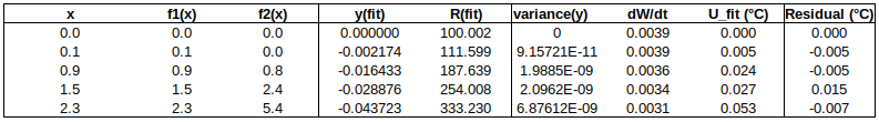
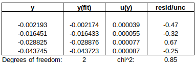
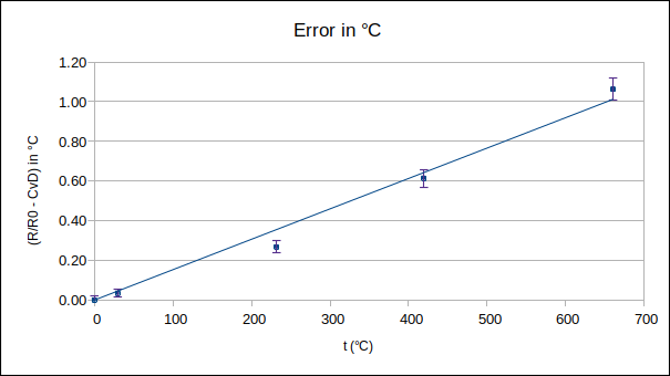
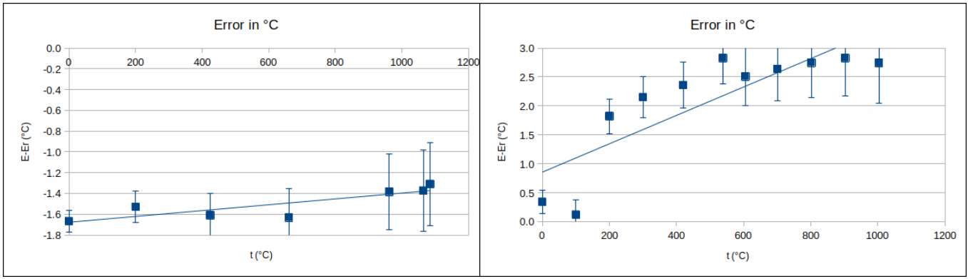
Now to check the fitted curve against the measured data (residual = measured – fitted):
Are the residuals small enough, or, does the model fit the data well enough, relative to the uncertainties?: The chi-squared statistic, chi^2 = [(residual_1/u1)^2 + (residual_2/u2)^2 + …], will tell us:
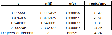
Chi-squared is larger than the degrees of freedom (= number of data points – number of fitted parameters = 4-2), so either the uncertainties are underestimated, or the model does not represent the data well (relative to the uncertainties). If chi^2 ≲ d.o.f., then the fit is “good enough”. (This is only strictly true if the uncertainties at different points are uncorrelated, but we will assume that this is the case.)
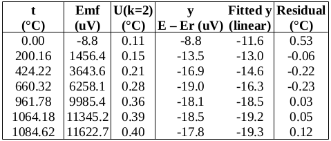
DEVIATION FROM ITS-90 REFERENCE FUNCTION
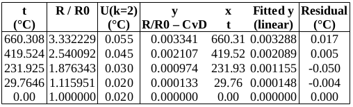
Perhaps direct fitting to the Callendar equation is not good enough, at this level of uncertainty. Let’s try deviations from the ITS-90 reference function – the reference function should take care of much of the PRT’s non-linearity, leaving us with smoother data to fit.
For the range 0 to 660 °C, the ITS-90 document gives the deviation function as: W-Wr = a∙(W-1) + b∙(W-1)^2 + c∙(W-1)^3, where W = Rt/Rtp and Wr is the value of the reference function.
It is good practice in curve fitting to use as few coefficients as will adequately fit the data, so we will try two, a and b.
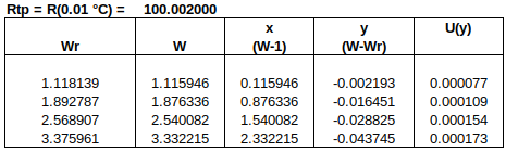
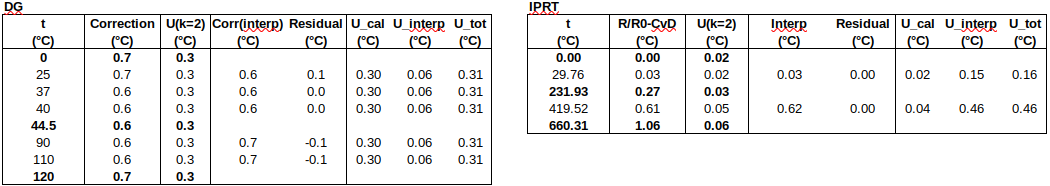
Now to check the fitted curve against the measured data (residual = measured – fitted):
It can be seen that this fit is better than the previous one. (Residuals are around half the size.)
Chi-squared is smaller than the degrees of freedom, indicating that the curve fits the data well, within the uncertainties.
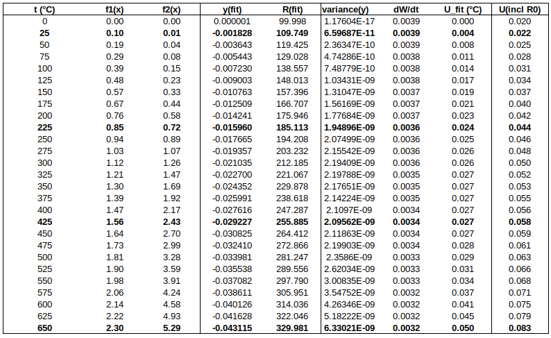
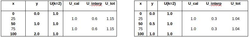
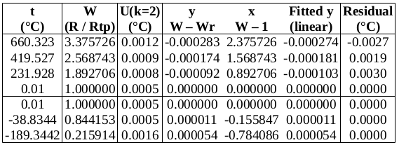
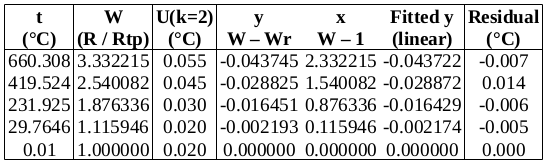
Below is a table of fitted values. Because of the structure of the ITS-90 functions, the uncertainty of the curve is zero at the water triple point (WTP, 0.01 °C). The uncertainty at WTP is added to the uncertainty of the curve, in the rightmost column.
CONCLUSIONS
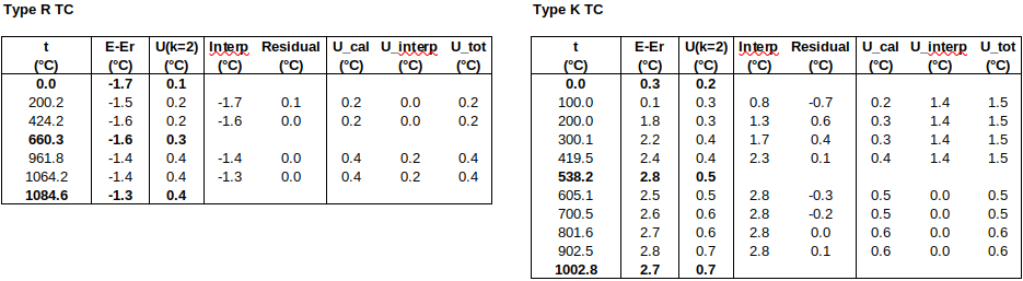
∙Both curves, fitted directly to measured PRT data, and to deviations from a reference function, represent the behaviour of the UUT better than do the individual data points. (The curves take into account all the data points, thereby potentially “smoothing out” random errors in measurement.)
∙The ITS-90 deviation function fits the data better, as is expected when using a good reference function.
∙When weighted least squares fitting is performed, the covariance matrix provides a statistically justified manner of propagating uncertainty to intermediate points, which results in small uncertainties. (To be strictly correct, we should have considered possible correlation between data points, but, as long as the dominant uncertainty component(s) are uncorrelated, our approach is reasonable.)
(Contact the author at LMC-Solutions.co.za.)
 , similar to the formula for the
  .
.
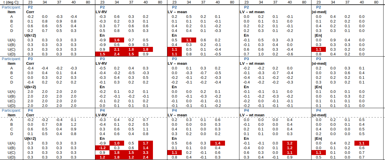
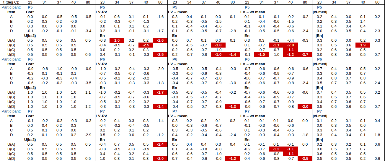
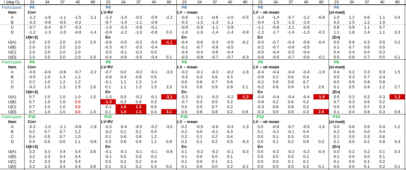
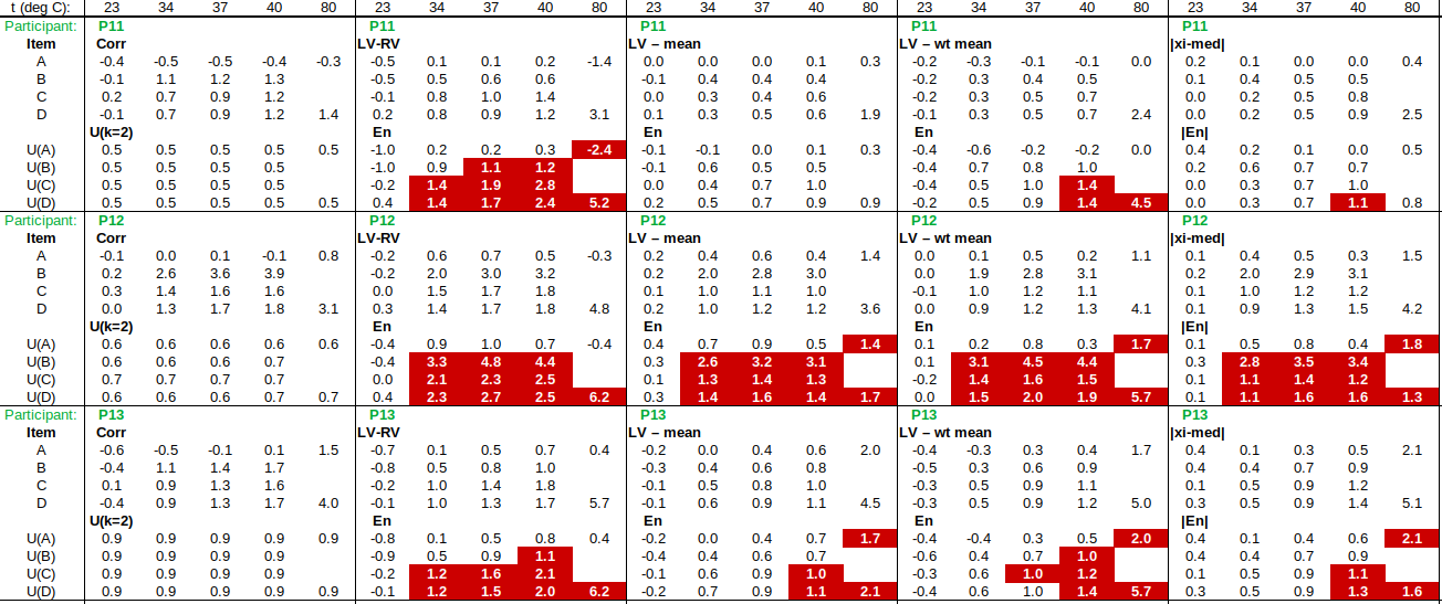
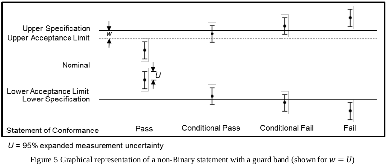
 , also called Reference Value, RV), which should represent the “true” value (traceable to the relevant SI unit(s)), within a particular uncertainty (
 or U(RV)). The goal is to demonstrate “equivalence to the SI”, within a certain uncertainty. In practice, this often becomes “equivalence to some reputable laboratories performing such calibrations”, or “equivalence to some other laboratories performing such calibrations”.
 , which would then be RV. The variance of the weighted mean is given by
  . The benefit of this approach is that, if participant uncertainties are reliable, they are taken into account appropriately in forming both RV and U(RV). (The approaches in b), below, do not take estimated uncertainties into account at all, only the spread of results.) The drawback of the weighted mean is that U(RV) does not include any factors arising from instability/drift of the ILC item (which would only become apparent during circulation of the item).
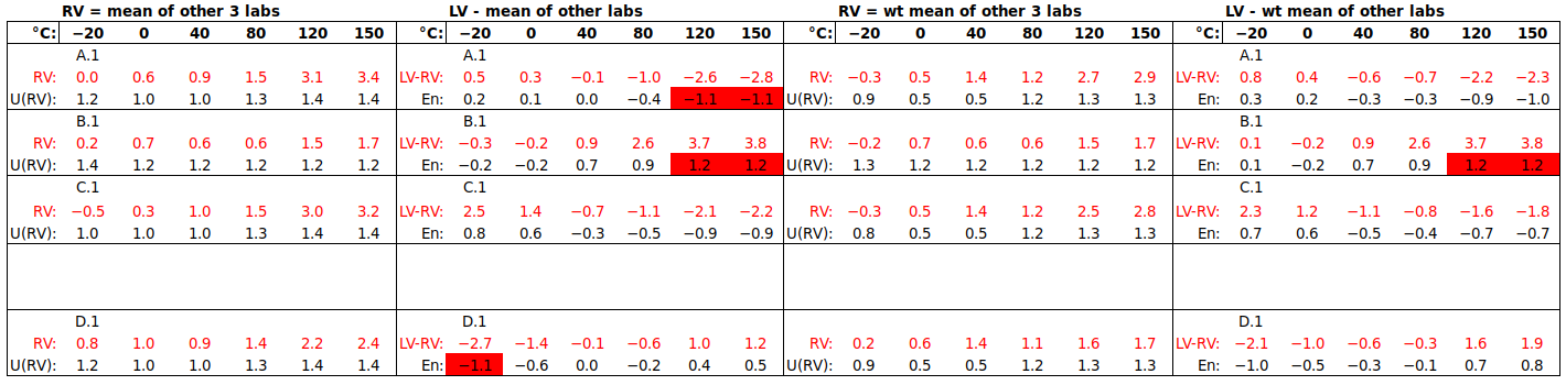
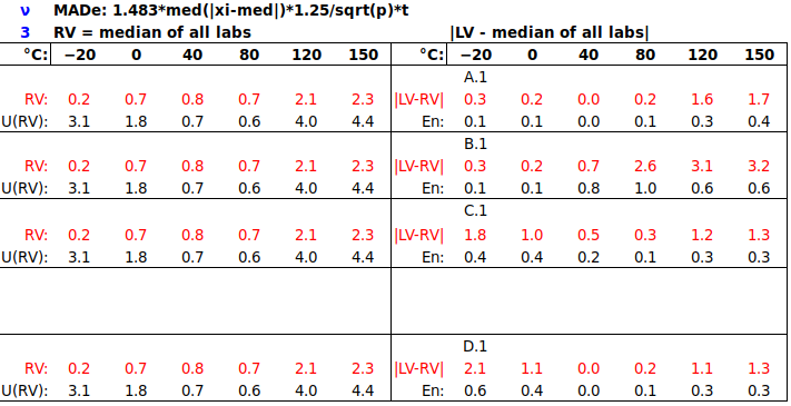
 are sorted in increasing order. Its standard deviation may be estimated by the scaled median absolute deviation (MADe), which is calculated as follows [13528 clause C.2.2]:
 , as follows [13528 clause 7.7.3]:
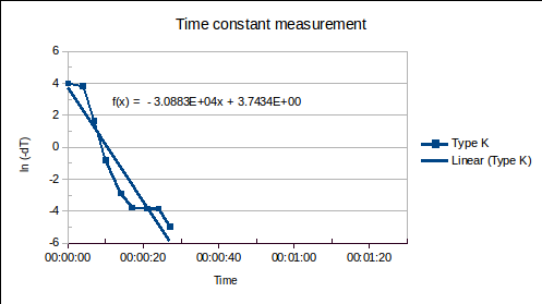
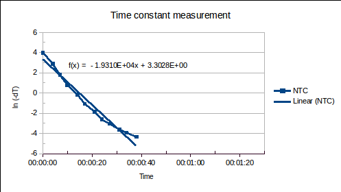
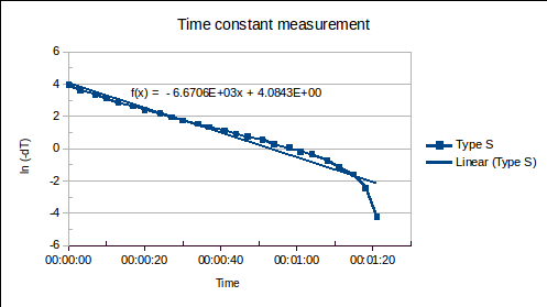
 (1)
(1) is the time since the sensor was plunged into an environment of temperature
  ,
,  is the initial temperature of the sensor, and
  is the time constant.
 , of the sensor and the heat transfer coefficient,
  , from environment to sensor:
  . It may be determined by measuring
  versus
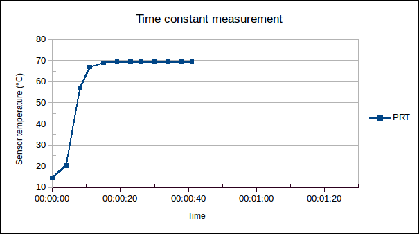
 (1a)
(1a)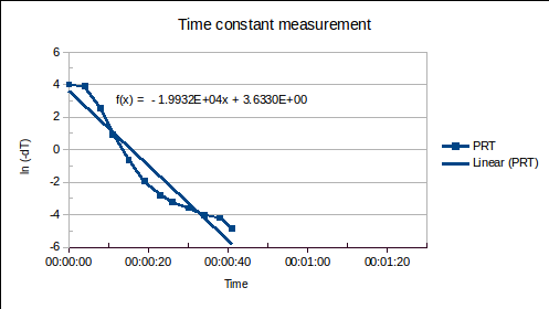
 , where
  is the number of readings.)
 .
. is the combined mass of the piston, sleeve (weight carrier) and the weights used. The uncertainty of calibration may be
  (around
  , may be measured to better than
  , in which case its uncertainty is negligible. However, if it is estimated by a
  may be
  , which is significant. The certificate typically reports
  uses conventional air and weight densities (1.2 kg.m^-3 and 8000 kg.m^-3), not the actual ones. The buoyancy correction is around
  : the additional
  for deviation from conventional air density, and its uncertainty, is often negligible (
 below 300 m altitude).
 , is unimportant for pneumatic systems. For hydraulic ones, the contribution to total weight may be
  , important to correct for, but whose uncertainty has a negligible effect.
 , has an uncertainty around
  : this is usually the dominant component of total DWT uncertainty, especially at high pressures. The pressure distortion coefficient,
  , is ~
 per MPa, i.e., the correction goes up to
  at 500 MPa. Say its uncertainty is 10% of its value, i.e., up to
  at lower pressures. The thermal expansion coefficient,
  , is ~
 per °C. So, for
  ~1 °C, the contribution to
  is around
  is ~1000 times smaller than for oil, the head correction,
  , is often negligible. The uncertainty in the head correction is typically dominated by
  , i.e.,
  and
and  are negligible. If h~0.27 m (as in the Fluke P3830 pressure balance) and
  , one of the two largest contributors. At higher pressures, the
  term dominates and U(head) becomes less important (e.g.,
  contribution to
  (sensitivity coefficient =
  )
) (sensitivity coefficient =
  )
) )
) )
) . The absolute accuracy of the balance used to weigh the dishes is not important, nor are the absolute times indicated by the watch: only the changes are of interest.
 ? We could evaluate the sensitivity of the balance [
 , or 27%. Note that this is significantly worse than the balance sensitivity of 1% of total mass gain (which would translate to 0.000 001 g/h) required in the test methods [E96 clause 6.3, 952-1 clause 6.11.4.2.2], indicating that balance sensitivity is, in this case, negligible compared to other factors causing “noise” in the mass readings. It highlights the importance of having more data points than unknowns and performing a least squares fit, as this uncertainty component would otherwise be grossly underestimated. It also shows how the standard error in the slope is far more useful than the correlation coefficient R^2, in quantifying uncertainties.
 ? (In the previous paragraph, it seems we already obtained a “complete” uncertainty for the slope. However, the fitting procedure we used assumes no uncertainty in the x-values, only uncertainty in the y-values, so we had better look at the uncertainty in the time intervals, too.) The documentary standards require time intervals to be measured to an accuracy of 1% (for example, a 24 hour interval to an accuracy of 15 minutes), so,
  [E96 clause 11.3, 952-1 clause 6.11.4.2.2]. We can see that the relative uncertainty in
  . When parameters are combined by simple multiplication or division, the relative uncertainties may be added simply in quadrature. So,
  . As
. As  is typically smaller than 0.01, it, like
  , can be neglected, so that the final relative uncertainty is
  , or 27%. In other words, U(k=2) = 1.00 g/m^2/24h * 0.27 = 0.27 g/m^2/24h.
 . If the uncertainties are quite different, the weighted mean (giving more weight to those specimens with smaller uncertainties) could be used:
  . The uncertainty of the weighted mean is
  , which also works out to be 0.16 g/m^2/24h, in the above example.