ABSTRACT
Calibration laboratories must often organise their own interlaboratory comparisons (ILCs) to evaluate/monitor their performance, as “in the field of calibration very few regularly organised PT schemes exist” [EA-4/18, “Guidance on the level and frequency of proficiency testing participation”, 2021]. Accreditation Bodies (ABs) will typically assess such a laboratory against “relevant elements” of ISO/IEC 17043. This article will discuss which of these elements are relevant to an ILC organiser (PT provider) and to an ILC participant, in the field of calibration. It also discusses how the assigned value (Reference Value) and its uncertainty may be estimated, focussing on small ILCs.
INTRODUCTION
(Clause numbers from ISO/IEC 17043:2023 are given below, for convenience.)
A calibration laboratory may often decide to organise an ILC itself, as
(i) the parameter it wishes to evaluate is not addressed by any scheme offered by a local accredited PT provider, or
(ii) the range or particular points of interest to the laboratory are not included in available PT schemes, or
(iii) the uncertainty achievable by available PT schemes may be unacceptable, owing to lengthy circulation or characteristics of the artefact, or
(iv) the time before receiving the results from an available PT scheme may be too long to meet the laboratory’s needs.
Note: The terms “PT” and “ILC” are used interchangeably in this article – commercial calibration laboratories almost always participate in ILCs for the purpose of evaluating their performance, so such ILCs would typically be classified as “PT”, according to the Introduction of 17043. Also, as most self-organised PT involves seven or less laboratories, it would usually be classified as “small ILC” according to the EA definition. (As ILCs are intended to compare results between laboratories, we count the number of laboratories (having independent measurement standards, equipment, etc) that participate, not the number of metrologists submitting results.)
If a calibration laboratory being assessed by an AB is the ILC organiser (PT provider), they will be expected to comply with some clauses of 17043 related to personnel (6.2), design and planning (7.2), stability of ILC items (7.3), evaluation and reporting (7.4), etc.
If the lab is merely a participant, they will be assessed on the content of the PT report (7.4.3) and the fitness-for-purpose/appropriateness of the ILC (performance of the lab and criteria used to evaluate performance).
Note: Regarding those clauses applicable only to a PT provider (ILC organiser), a PT participant may still be required “to ensure that the organiser … fulfils the relevant requirements” [EA-4/21, “Guidelines for the assessment of the appropriateness of small interlaboratory comparison within the process of accreditation”, 2026, section 5].
ASSIGNED VALUE (REFERENCE VALUE)
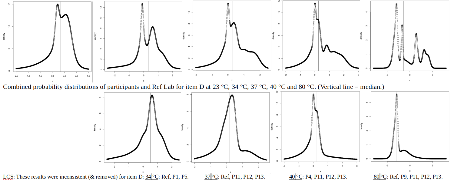
(i) If the assigned value of the ILC item (also called Reference Value, RV) is obtained externally, from one non-participating laboratory, the ILC is, in effect, a series of bilateral comparisons, of each participant with the Reference Lab. The credibility of the Reference Lab is critical, and, as has been shown in a previous article, may not be taken for granted.
(ii) If RV is obtained from one ILC participant, it is effectively the same situation as in (i).
(iii) If RV is a consensus value, the following approach is recommended:
a) only one result per laboratory to be included in RV, to avoid biasing RV towards labs with many participating metrologists, and
b) exclude a laboratory’s own result from the RV to which it is compared, to avoid it biasing RV “towards itself” (especially for a small number of participants), and
c) use the simple (not weighted) mean as RV, since many laboratories’ accredited CMCs are not proportional to their capabilities, but arise, for example, from one ILC of many years ago, or from a very conservative uncertainty budget, or from the modest accuracy needs of their clients, not from the real capabilities of their equipment and method.
Must an ILC evaluate the difference between the participant’s result and the “true value”, or is it sufficient to demonstrate equivalence between participants?:
17043 clause 7.2.3.2 requires that “PT schemes in the area of calibration shall have assigned values with metrological traceability.” If each of the laboratories uses a calibrated reference standard and makes a credible uncertainty estimate, then RV may be obtained from one laboratory or from a consensus of several: in both cases, “the result can be related to a reference through a documented unbroken chain of calibrations, each contributing to the measurement uncertainty” [VIM], so it is traceable.
One might argue that the purpose of the ILC is to evaluate performance, so one cannot assume that a participant’s uncertainty estimate is credible. However, let’s consider the case where RV comes from an external laboratory: in effect, the ILC is a series of bilateral comparisons, of each participant with that external laboratory. All that is proven is equivalence between each participant and the Reference Lab. In some cases, the Reference Lab may use a “reference method” [ISO 13528:2015 clause 7.5.1], but, in the calibration domain, the Reference Lab is usually one that reports a smaller uncertainty than any of the participants, while using the same method as they do. As the external laboratory’s traceability is not fundamentally different from that of an ILC participant, if an external RV has traceability, so does one calculated from participants’ results.
In the strict sense, all any ILC ever proves is equivalence – we rely on certain assumptions to relate this equivalence to “competence”, or agreement with the “true value”. These assumptions are:
(i) the laboratories contributing to RV are “determined to be reliable, by some pre-defined criteria, such as accreditation status or on the basis of prior performance” [13528:2015 clause 7.7.1.1], and
(ii) RV does not “include unknown bias due to the general use of faulty methodology … not reflected in the … uncertainty” [13528:2015 clause 7.7.1.4 b)].
The first assumption may be satisfied by choosing an external lab, or subset of participants, whose reliability is supported by historical performance. (As mentioned above, this is not fool-proof.)
The second assumption, that there is no common bias in the results contributing to RV (which would not be evident in the spread/dispersion of these results), is more justified, the greater the variety of equipment and variations in method that are applied by laboratories contributing to RV. So, the more independent contributors to RV, the better.
It does happen, even in Key Comparisons at NMI level, that common bias is only discovered by the “discrepant” results of a few laboratories (for example, in CCT-K7 of 2004, three out of 21 participants were “correct”), so neither the size nor the level of the ILC can completely remove the risk of bias.
In ILCs in the calibration domain, we do not realistically aim to prove anything more than equivalence to a credible Reference Value, no matter whether that Reference Value originates from one laboratory or several, participants or not.
Understanding that a PT Reference Value, unlike a Key Comparison Reference Value (KCRV), is not intended to be the best estimate of the SI value of the measurand, it is easier to accept the concept of a different consensus Reference Value for each ILC participant, which is the approach recommended by this author in (iii) b) above and in a previous paper.
The way in which the Reference Value and its uncertainty are estimated is critical to the value of any ILC, especially small ILC using a consensus value, where the “small dataset makes it challenging to accurately identify the distribution of the data and to reliably detect outliers” [EA-4/21:2026 section 4.1].
However, remembering that the ILC’s “modest” goal is to demonstrate equivalence with a credible Reference Value, within the reported uncertainty, the following approach is recommended (considering a comparison between four laboratories, A to D), if a consensus value is to be used:
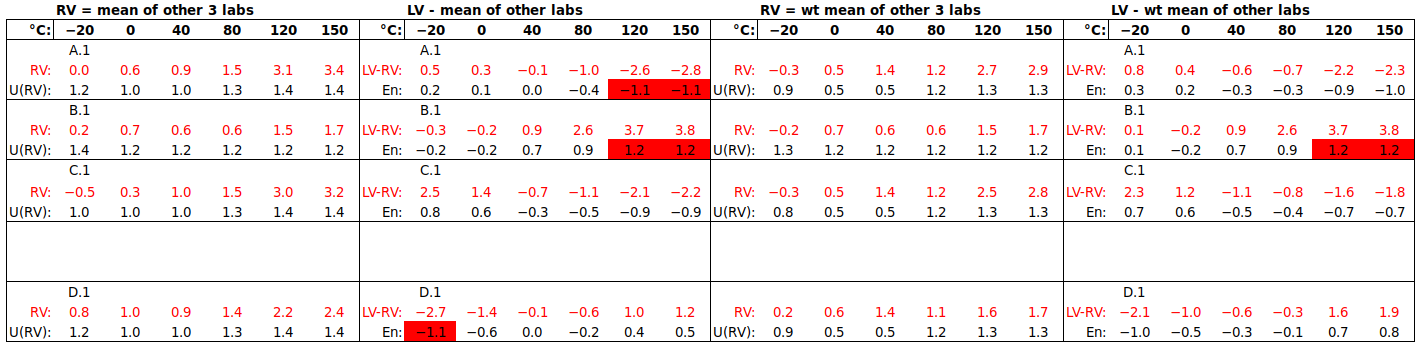
(i) For laboratory A, use RV = mean of one result each from laboratories B, C and D. If more than one metrologist from each lab submits a result, the lab must decide which one of its results will contribute to RV, before having sight of other labs’ results.
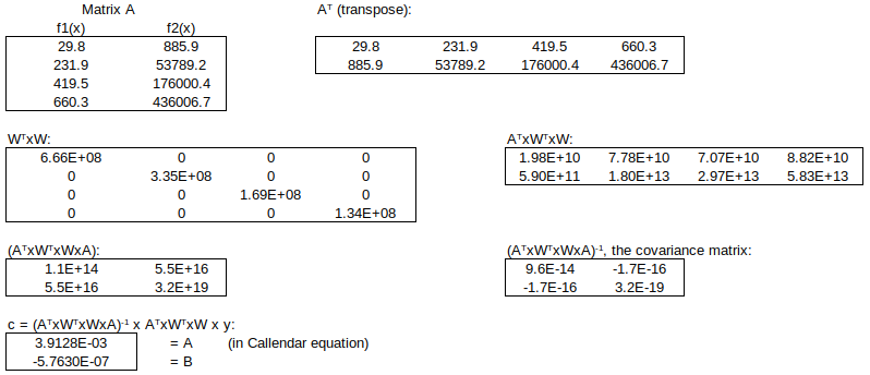
(ii) For laboratory A, use U(RV) = 1/3∙√[U(B)^2 + U(C)^2 + U(D)^2]. This formula for the uncertainty of the (unweighted) mean may be understood by analogy with the standard deviation of the mean: if U(B) = U(C) = U(D) = U, then U(RV) = 1/3∙√[3U^2] = 1/√3∙U, i.e., the uncertainty is divided by the square root of the number of results.
Do not use the spread of participants’ results as U(RV), as the goal is to demonstrate equivalence within the reported uncertainties.
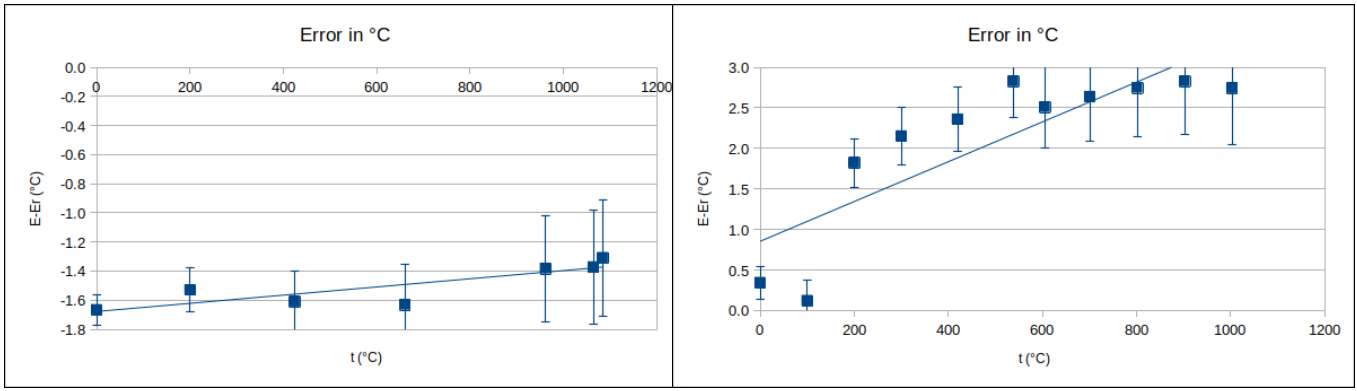
If an uncertainty component related to artefact drift must be added, this should be evident from stability checks performed at the start and end of the ILC, or other evidence of stability included in the ILC report. If, after consideration of possible artefact drift, the resultant uncertainties U(RV) and U(LV) (U(A), U(B), U(C) or U(D)) do not account fully for the observed spread of results (“over-dispersion”) [13528:2015 clause 7.6.3 c)], this may be interpreted as a failure, on the part of the organiser or participants, to identify all relevant uncertainty contributors.
(The ILC protocol, or instructions for participants, should specify all conditions that might significantly affect the comparability of results. Over-dispersion is a sign that one or more parties neglected or under-estimated some such factors.)
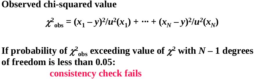
(iii) Calculate the normalised error, En, in the usual way, and consider |En| ≤ 1 to be acceptable.
In the case of a bilateral comparison, the above approach reduces to: RV for participant A is participant B’s result (with its uncertainty), and vice versa. If the participants’ uncertainties are similar, a bilateral comparison evaluates the performance of both participants. If U(A) is significantly smaller than U(B), then only participant B is rigorously evaluated.
May the uncertainty of the Reference Value, U(RV), be larger than the laboratory’s reported uncertainty, U(LV)? In South Africa, yes: there is no regulation mandating U(RV) ≤ U(LV), nor, in fact, how often an ILC should be performed to CMC. This is perhaps not unreasonable – for labs having the smallest CMCs in the country, insisting that every ILC test CMC may be onerous. But, at least in preparation for the initial assessment, |LV-RV|, U(LV) and U(RV) should be smaller than or equal to the lab’s proposed CMC. And, after any change in the lab’s measurement standards, equipment or method that might significantly change the achievable uncertainty, the lab should test CMC somehow, preferably by ILC.
ILC ORGANISER (PT PROVIDER)
The following clauses of 17043 should be addressed by an ILC organiser:
If the organiser is a 17025-accredited lab, then 4.1 Impartiality, 4.2 Confidentiality and 5. Structural requirements are already addressed elsewhere, and need not specifically be addressed in the context of PT.
6.2 Personnel should be competent and authorised to organise ILCs. “it is preferable for the personnel performing the measurements not to overlap with those organising the ILC. To prevent collusion, the ILC organiser should ensure that personnel performing measurement are not informed in advance of … assigned values” [EA-4/21:2026 section 5.2.1]. In small labs, overlap between the organiser and participant may be unavoidable. In such cases, the organising lab should preferably perform measurements before the lab(s) providing RV.
In an accredited cal lab, 6.3 Facilities should be addressed elsewhere.
6.4 Externally provided products and services: If RV is provided by an external lab, criteria for choosing such a lab should be documented.
In an accredited cal lab, 7.1 Contract review should be addressed elsewhere.
7.2 Design and planning: This is a “key focus of the assessment” [EA-4/21:2026 section 5.3.2].
7.2.1.3 The PT provider plan and/or instructions for participants (ILC protocol) should address the following:
a) Main contact person. If organised jointly, the list of persons or CABs involved.
d) List of participants.
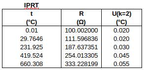
e), f), g) The measurand or characteristic to be determined: All factors that must be harmonised between participants, to ensure comparability of results, should be specified. For example, for an infrared thermometer, the size of and distance to the target should be specified, as well as the preset emissivity of the thermometer (if not obvious).
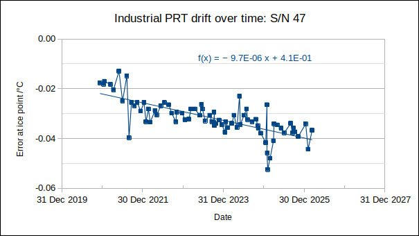
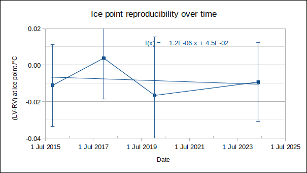
h) Quality control (stability checks) required for the ILC item (also addressed in 17043 7.3.2): If the artefact should return to the organiser for periodic intermediate checks, the frequency of such checks should be planned. For example, a PRT may require an ice point check after visiting every participant.
j), k) Timeframe of the ILC: When each participant is scheduled to measure, deadlines for submission of results.
l) Handling, preparing, measuring and shipping (also addressed in 17043 7.3.3-4): How the artefact should be handled, prepared for measurement, measured and transported. Information on the method(s) or procedures to be used by the participants.
n) Description of the reporting format for participants.
o), p), r) Description of the method for evaluating the comparability of the results, including statistical analysis and criteria used for performance evaluation. See the discussion of ASSIGNED VALUE (REFERENCE VALUE), above. Discussed further in 17043 7.2.2 and 7.2.3.
s) Reporting format from the ILC organiser.
t) Confidentiality: Results should be anonymised in the report, unless the participants waive confidentiality.
7.3.5 Instructions for participants: See 7.2.1.3 e), f), g), j), k), l), n), above.
7.4.3.2 The PT report should include:
Date of the ILC.
a) Name and contact details of ILC organiser.
g) Identification of the small ILC scheme or round.
h) Description of the ILC item, including how the stability of the ILC item was determined.
i) Participants’ results.
j), k), l), m) Method for evaluating RV and U(RV), and their resultant values.
p) Participants’ performance.
s) Comments and recommendations based on the outcome of the ILC.
In an accredited cal lab, 7.5 Records, control of data, ensuring validity of results and non-conforming work, 7.6 Complaints and 7.7 Appeals should be addressed elsewhere.
8.8 Internal audit and 8.9 Management review should include self-organised ILCs.
ILC PARTICIPANT
The lab’s PT participation plan should determine the level and frequency of ILC participation via a risk analysis, considering [EA-4/18]:
∙use of internal quality control measures, such as intermediate checks
∙number of measurements undertaken
∙turnover of technical staff
∙experience and knowledge of technical staff
∙source of metrological traceability
∙known stability/instability of the methodology
∙unsatisfactory results in past PT
The performance of the lab, and criteria used to evaluate performance, as documented in ILC reports, will be assessed.
CONCLUSIONS
∙The purpose of PT/ILC for commercial calibration laboratories is concluded to be: to demonstrate equivalence with a credible Reference Value (RV), within reported uncertainties.
∙For RV to be credible, it should be determined from (i) the results of reputable laboratories, (ii) in a mathematically appropriate way.
∙Avoiding bias in RV is especially important for small ILCs: only one result per laboratory should contribute to RV, and the laboratory being evaluated should be excluded from the RV to which its result is compared.
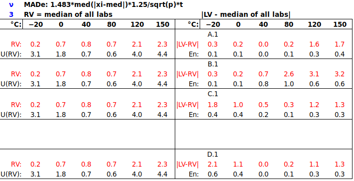
∙The uncertainty of the Reference Value, U(RV), should be determined from participants’ uncertainties, not from the spread of results, as the goal is to demonstrate equivalence within reported uncertainties. (This makes it difficult to use the median and Median Absolute Deviation, MADe, as RV and U(RV).)
∙A consensus Reference Value may be as metrologically traceable as one from an external laboratory.
∙For a consensus RV, the mean is preferred over the weighted mean, as participants’ reported uncertainties may vary widely, without technical justification.
∙A PT provider (ILC organiser) should have:
– personnel that are competent in the technical domain of the ILC and in statistical analysis of results,
– a PT provider plan and instructions for participants (protocol) that carefully define the measurand and conditions of measurement (so that results are comparable), and plan appropriate intermediate checks on ILC artefacts,
∙A PT participant should ensure
– that their PT participation plan plans the frequency of ILC participation in consideration of risk mitigating or enhancing factors present in their laboratory,
– that the ILCs they participate in do support their required performance (CMCs).
Contact the author at LMC-Solutions.co.za
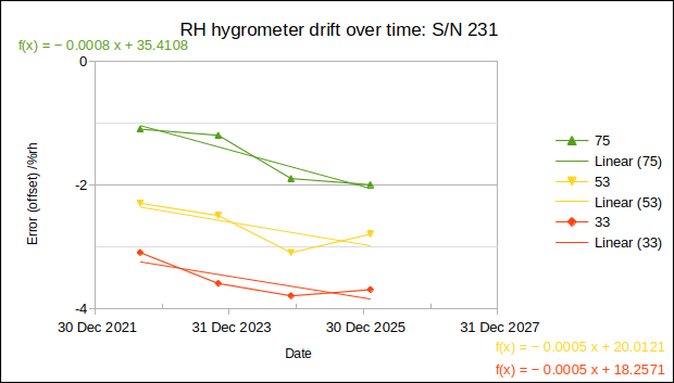
![High-quality RH hygrometer drifts 0.0005 %rh/day or 0.2 %rh/year [Jonker et al, "The Humidity Calibration Facility of the National Metrology Institute of South Africa (NMISA)", Int J Thermophys, 2008].](http://metrologyrules.com/wp1/wp-content/uploads/2026/04/Drift_RH_HMS-530_NMISA_trend.png)
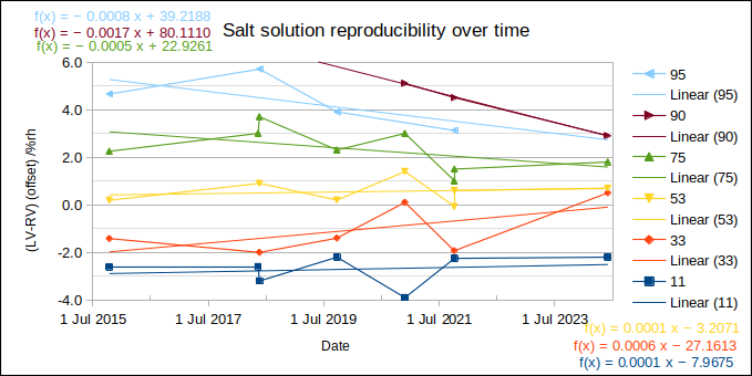
![Saturated salt solution capsules drift by less than 0.5 %rh over four years, or 0.1 %rh/year [Jonker et al, "The Humidity Calibration Facility of the National Metrology Institute of South Africa (NMISA)", Int J Thermophys, 2008].](http://metrologyrules.com/wp1/wp-content/uploads/2026/04/Drift_saturated_salt_capsules_NMISA.png)

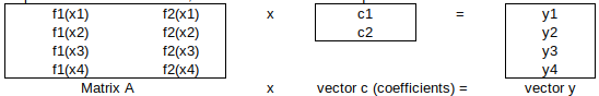

 , similar to the formula for the
  .
.