For a Temperature calibration laboratory, a testing laboratory or any other business that needs to verify the accuracy of its thermometers, the ability to realise the ice point is perhaps the most important and most basic of Thermometry capabilities.

Q: What are some of the uses of the ice point?

A: 1. Intermediate checks of resistance thermometers (PRTs and thermistors) and liquid-in-glass thermometers:

Some method of verifying the accuracy of measuring equipment between calibrations is usually required by a quality management system, so that the equipment’s reliability can be checked when necessary, preferably without the inconvenience of using an external calibration service. It is possible to compare a thermometer to another of similar or greater accuracy, but using an “absolute” measurement standard like the ice point is often more convenient. (The ice point can be realised to an accuracy of about ± 0.01 °C without too much trouble.)

Note: Measurement at the ice point is not a very sensitive in-service check for thermocouples. For a PRT, a change from 100.0 Ω to 100.1 Ω (0.25 °C) at 0 °C is equivalent to a change from 300.0 Ω to 300.3 Ω (0.75 °C) at 550 °C, but, for a type K thermocouple, a 10 µV (0.25 °C) change at 0 °C is equivalent to a 260 µV (7 °C) change at 550 °C. This makes it necessary to check thermocouples at a temperature further from ambient (for example, at 200 °C) to draw meaningful conclusions about drift.

2. Recalibration of liquid-in-glass (LIG) thermometers:

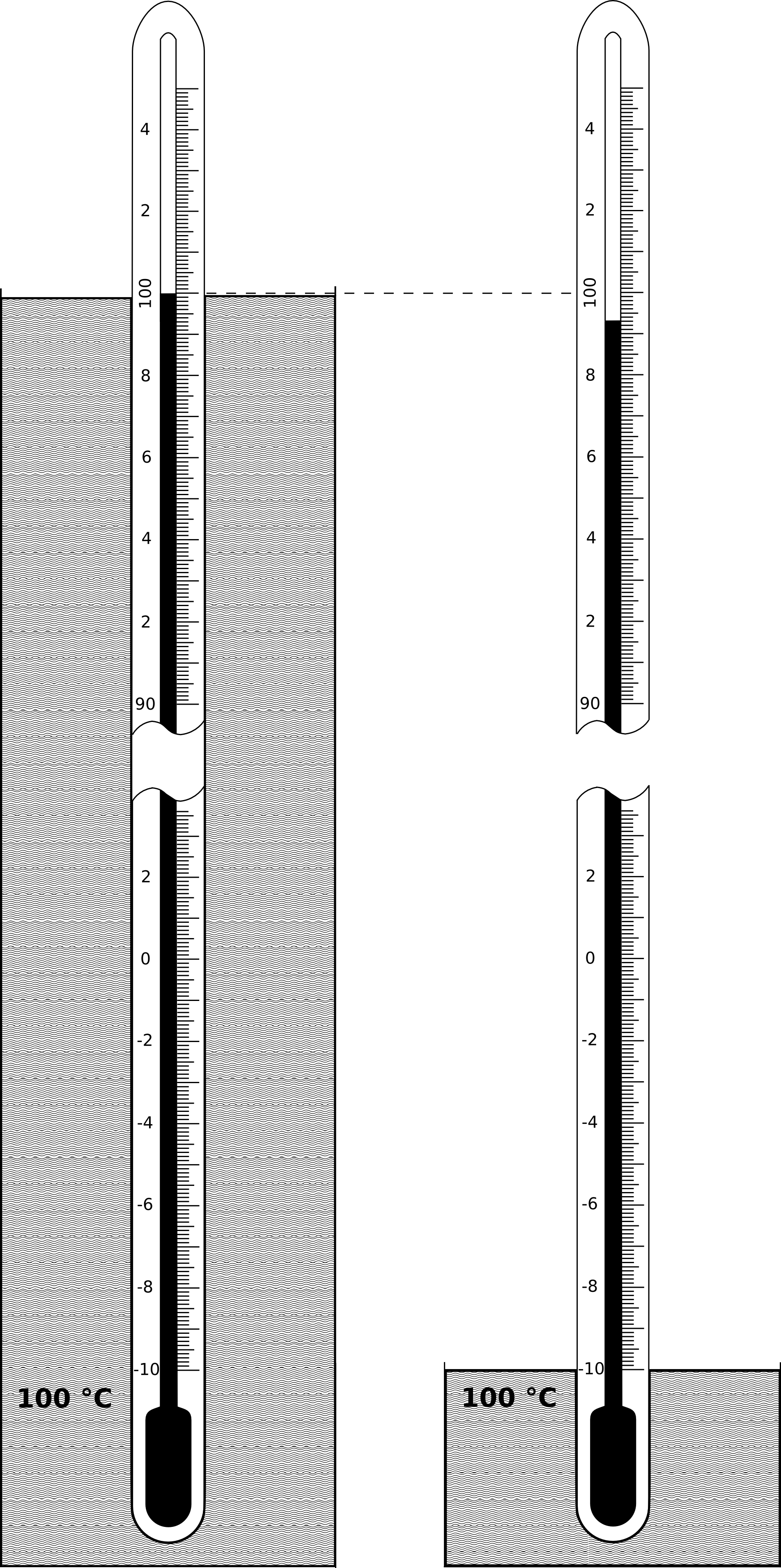
If a LIG thermometer is not used above 200 °C or so, all significant changes in calibration will be due to changes in bulb volume, not to changes in the capillary [Cross et al, Maintenance, Validation, and Recalibration of Liquid-in-Glass Thermometers, NIST SP 1088, 2009]. (We do not consider gross errors, such as a separated liquid column, here.) The effect of such changes in the bulb (for example, secular change and temporary depression of zero) may be evaluated by observing the temperature indicated by the thermometer at the ice point. (Comparison with a calibrated reference thermometer of equal or greater accuracy, in a uniform-temperature environment, is also an option, but the ice point is often simpler.) Past calibration results for the thermometer may then be adjusted by a constant offset, to compensate for the difference between the present and past indicated temperatures at 0 °C. (For example, if the reading at 0 °C rises from -0.4 °C to -0.3 °C, the reading at 100 °C will also rise by 0.1 °C.) This single-point recalibration technique, combined with regular visual inspection to identify problems such as a separated liquid column, is often sufficient to assure the quality of measurement results, avoiding the need for expensive and time-consuming recalibration at an external calibration laboratory.

(Note: We must evaluate how well we can realise and use an ice point, before relying on it unreservedly. To do so, measure a thermometer at the ice point yourself, immediately before and/or after it returns from calibration, and compare your result(s) to that reported in the calibration certificate. Repeat this check periodically, to evaluate reproducibility. Bear in mind the uncertainty of calibration and the accuracy to which you can read the thermometer, when interpreting the results.)

3. Calibration or intermediate checks of low-temperature infrared radiation thermometers:

The emissivities of ice and liquid water at infrared wavelengths longer than 2 µm are high (~0.96), making it easy to create a blackbody target (emissivity ≈ 1) for calibration of low-temperature infrared radiation thermometers. (Such thermometers usually operate in the wavelength range 8 to 14 µm.)

Note: When aiming the thermometer at the ice point, take care to view an area of melting ice. The top surface of the ice may often not contain liquid water, and may be at a temperature colder than 0 °C: rather make a hole in the ice and view an area of grey slush, lower down. The hole also increases the effective emissivity of the target.

4. For a reference PRT in a calibration laboratory, adjustment of its calibration results to compensate for drift:

If a PRT is bumped and its resistance increases, the relative change in resistance is usually similar over the whole temperature range. For example, a change from 100.0 Ω to 100.1 Ω at 0 °C (a 0.1 % increase) will usually mean a change from 300.0 Ω to 300.3 Ω at 550 °C (again, a 0.1 % increase). If the calibration certificate reports a curve of resistance as a function of temperature, it will usually be written in terms of a resistance ratio, R(T)/R(0.01 °C) or R(T)/R(0.00 °C). If the user can measure R(0.00 °C) sufficiently accurately, he may use his latest measurement at the ice point to calculate the resistance ratio, thereby compensating for much of the drift in R(T) since the PRT’s calibration.

Notes:

(i) To calculate R(0.01 °C) from the measured resistance at the ice point, R(0.00 °C), use R(0.01 °C) = R(0.00 °C) / W(0.00 °C) = R(0.00 °C) / 0.99996.

(ii) If the user uses his own measurement of R(0 °C) in the calculation of resistance ratio (and, subsequently, temperature), he must include the uncertainty of that measurement in the uncertainty of the calculated temperature. For this reason, it is only sensible to use your own measurement of R(0 °C) to compensate for drift, if the uncertainty in that value is smaller than the typical drift for which you are trying to compensate.

5. For a  reference PRT measured on an ohmmeter or a resistance bridge, elimination of most resistance measurement errors:

If the PRT’s calibration results are expressed in terms of resistance ratio (as discussed above), the user can eliminate the effect of most errors in resistance measurement, by measuring both R(T) and R(0 °C) on the same range of the same measuring instrument. Then, the resistance ratio will be independent of any linear errors in the resistance measuring instrument, including, most importantly, any drift in a reference resistor or reference voltage since its last calibration. The only resistance measurement errors that still have an effect are those that are not proportional to the measured resistance value.

6. For a thermocouple, more accurate cold junction temperature:

The output of a thermocouple depends on the temperature difference between the measuring (or “hot”) junction and the reference (or “cold”) junction: any uncertainty in the reference junction temperature causes an uncertainty in the calculated temperature of the measuring junction. While electronic Cold Junction Compensation typically measures the temperature of the reference junction to an accuracy of ± (0.5 to 0.1) °C, immersing the reference junction in an ice point controls its temperature to 0.00 °C ± 0.01 °C, that is, an order of magnitude more accurately.

Q: How do we prepare an ice point?

A: The container in which the ice point is to be prepared should be thermally insulated. A wide-mouthed vacuum flask, 80 mm to 100 mm in diameter and 200 mm to 400 mm deep, is ideal. For convenience in cleaning the flask and packing the ice, it should not have a narrow neck. (It is convenient if you can fit your hand inside it.) If the thermal insulation at the bottom of the flask is good enough, a thermometer can be inserted all the way to the bottom without the tip being in a hot spot. (Vacuum insulation is better than expanded polystyrene.)

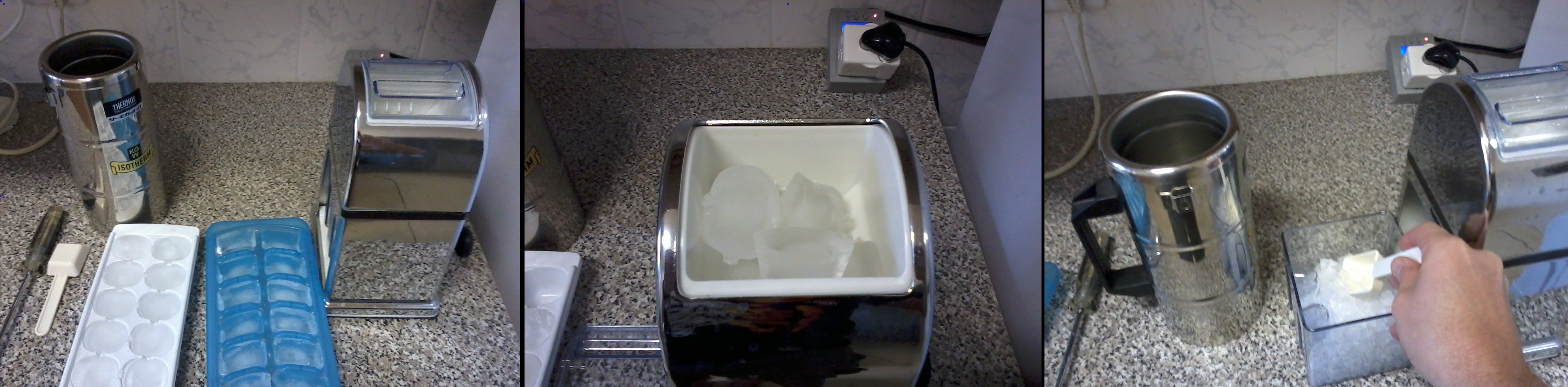
The ice to be used must be crushed or shaved, preferably to a chip size of 1 mm or less. It is preferable, but not essential, to make it from distilled or deionised water.

Sufficient liquid water should be available to fill approximately one third of the thermally insulated container. Again, distilled or deionised water is preferred, but tap water may be used.

A scoop will assist in handling the ice without contaminating it with salts from the hands.

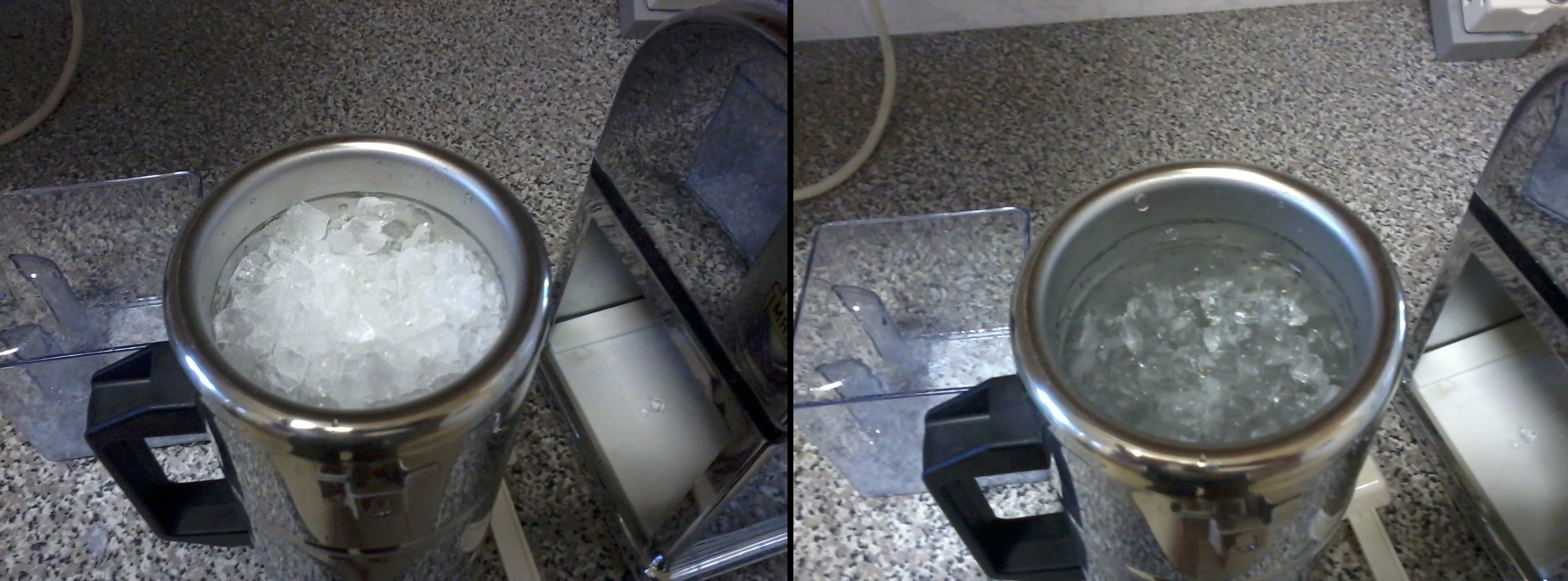
Scoop the crushed ice into the container, adding liquid water until the ice appears translucent or grey. (This indicates that it is melting, and therefore at 0 °C. White, frosty ice is usually colder than 0 °C.) Compact the ice, so that it is packed against the bottom of the container and is not floating on top of liquid water.

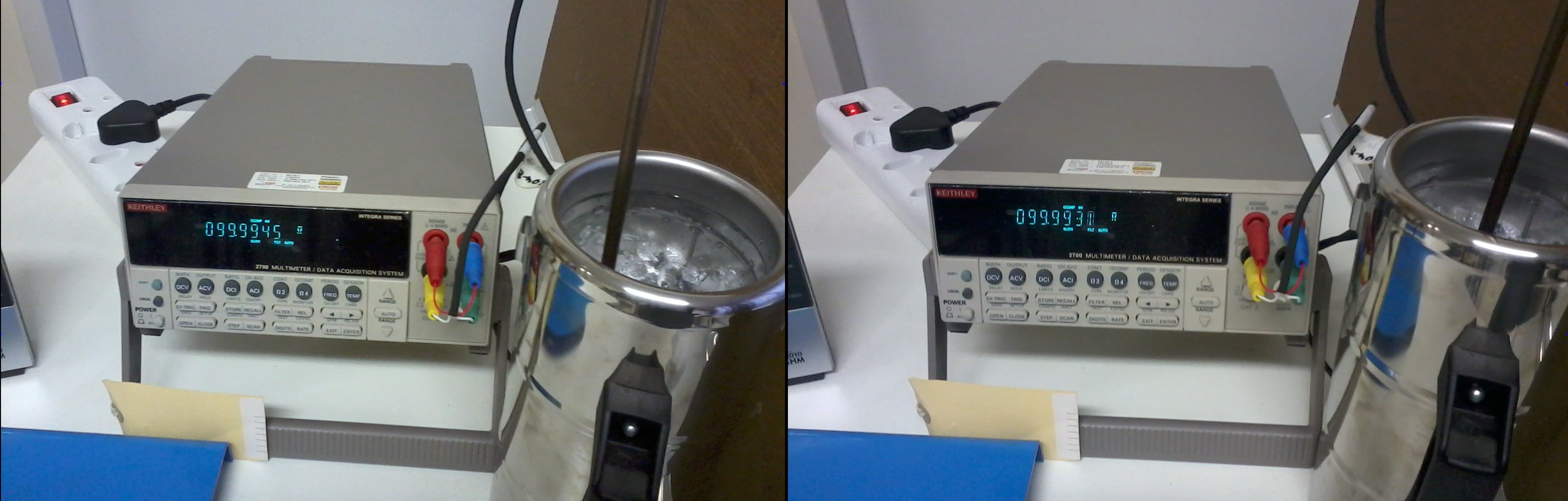
Insert the first thermometer to be measured, to the appropriate depth, wait 3 to 20 minutes for thermal equilibrium (five minutes is usually sufficient) and record its reading. When first realising the ice point, and periodically (perhaps monthly) thereafter, this thermometer should be one that has been calibrated to a high accuracy at 0 °C, to provide data on the deviation of your ice points from the desired temperature of 0.00 °C, and their stability in temperature.

Insert the next thermometer to be measured, ensuring that it is in good contact with the ice (particularly if you insert it in a previously used hole).

Drain off excess water when necessary, and re-compact the ice. (To determine how long it takes for an excess of liquid water to accumulate, insert a high-resolution thermometer to the bottom of an ice point and record its readings regularly over several hours, noting when they start to rise.)

(Contact the author at lmc-solutions.co.za.)

A liquid-in-glass (LIG) thermometer uses the thermal expansion of a liquid as the thermometric property. If the immersion depth of the thermometer in the medium of interest is changed from total to partial, the temperature of a part of the liquid column changes, its volume changes (because of thermal contraction or expansion), and the reading of the thermometer changes. (Note: This only happens if the medium of interest is at a different temperature from the surroundings. The further from room temperature is the medium of interest, the larger is the effect.)

Consider the mercury-in-glass thermometer in the sketch above: At total immersion, all of the mercury is at the bath temperature (100 °C) and the reading is 100.0 °C. When its immersion is reduced to the -10 °C mark, much of the liquid column is outside the bath (this is the “emergent” liquid column), at an average temperature somewhere between the bath temperature (100 °C) and room temperature (20 °C). (It is typically closer to room temperature than to the bath temperature.) Being at a lower temperature, its volume is less, and therefore the thermometer reading is lower (99.3 °C).

Q: Can we calculate how much the thermometer reading will change, with a change in immersion?

A: Yes, if we know the thermal expansion coefficient of the liquid (K), the length of the Emergent Liquid Column (N, expressed in °C on the thermometer scale), and the difference between the temperatures of the liquid column in the two cases (T[LC1] – T[LC2]). Then, the difference in thermometer readings between case 1 (total immersion) and case 2 (partial immersion) is K x N x (T[LC1] – T[LC2]).

The thermal expansion coefficient of mercury is K = 0.00016 per °C. (It’s about six times larger, 0.001 per °C, for ethanol.)

The length of the ELC in the partial immersion case is N = 100 °C – (-10 °C) = 110 °C. (To be precise, it is 109.3 °C, but an error of one percent is quite acceptable in such a calculation.)

In case 1 (total immersion), the liquid column is at the same temperature as the bath, that is, T[LC1] = 100 °C. In case 2 (partial immersion), we make a crude approximation, that the ELC is halfway between the bath temperature and room temperature, T[LC2] = (100 °C + 20 °C) / 2 = 60 °C. So, T[LC1] – T[LC2] = 40 °C. (As noted above, the actual average ELC temperature will be closer to room temperature than this crude estimate.)

Therefore, reading(1) – reading(2) = 0.00016 per °C x 110 °C x 40 °C = 0.7 °C.

Q: In which case is the thermometer reading higher? (Or, in which direction should we apply the ELC correction?)

A: In that situation where the liquid column is hotter, the thermometer reading will be higher. (In the above example, the reading will be higher in case 1, at total immersion.)

Q: In the above example, we determined the difference between readings at total and partial immersion. Can we determine the difference between two different partial immersions?

A: Yes. Such a calculation may be performed by correcting from partial immersion 2 to total immersion (let’s continue calling total immersion “situation 1″), then from total immersion to partial immersion 3. However, if we make the approximation that the differences in ELC temperatures (T[LC1] – T[LC2] and T[LC1] – T[LC3]) are equal, then we can calculate the difference between situations 3 and 2 directly, as K x (N[2] – N[3]) x (T[LC1] – T[LC2]).

For example, if the immersion depth in situation 3 was up to the 70 °C mark, then the difference in reading from situation 2 (immersion to the -10 °C mark) would be approximately 0.00016 per °C x (110 °C – 30 °C) x 40 °C = 0.5 °C. In such conversions between different partial immersions, it is particularly important to check the direction of the correction using common sense: as the liquid column is hotter in situation 3 than in 2, the reading will be higher by 0.5 °C.

Q: How accurate are such ELC corrections?

A: The thermal expansion coefficient (K) and length of the ELC (N) are usually known quite accurately (uncertainties of 2-4% at coverage factor k=2), but (T[LC1] – T[LC2]) might only be known with an uncertainty of 10% (k=2) if measured [Nicholas & White, Traceable Temperatures, p 275] or 50% (k=2) if crudely estimated as described above.

The best solution is to have the thermometer calibrated at the same immersion depth at which it is used. Even if the ELC temperature is not very accurately known, it is quite likely to be the same during calibration and during use, so that the calibration results can be applied by the user with a small uncertainty.

If calibration is performed at partial immersion, the calibration laboratory should estimate the average ELC temperature. The tips of two thermometers (LIG, thermocouple or PRT) may be placed at the surface of the liquid bath and at the top of the liquid column, respectively, and the average of the two measured temperatures used as the average ELC temperature. Although heat transfer may be quite different in the LIG thermometer and around the two other thermometers, this method may estimate (T[LC1] – T[LC2]) to an uncertainty of perhaps 20% (k=2).

It may be advisable for the calibration laboratory to report the uncertainty in average ELC temperature separately from other uncertainty components. In this way, the user can still benefit from a small uncertainty, if he uses the thermometer at the same immersion depth as that during calibration.

If the user must use the thermometer at an immersion depth significantly different from that during calibration, he must be prepared to accept an uncertainty of 10-50% (coverage factor k=2) in ELC correction, depending on how accurately the average ELC temperature is estimated. Using our crude estimation of T(LC2), the correction from case 1 to case 2 would be -0.7 °C ± 0.35 °C, at a coverage factor of k=2. If we had measured T(LC2), the uncertainty in the ELC correction might have been 0.14 °C (or 20%, in relative terms).

Exercises:

1. Calculate the reading at partial immersion (to the -10 °C mark) in the sketch above, if the thermometer liquid was ethanol (thermal expansion coefficient K = 0.001 per °C) instead of mercury.

2. Calculate the uncertainty in the ELC correction you have just determined for this alcohol-in-glass thermometer, if T[LC1] – T[LC2] = 40 °C ± 20 °C (coverage factor k=2).

3. An alcohol-in-glass thermometer reads -30.8 °C at total immersion. What is the reading if its immersion is reduced to the -50 °C mark and the average ELC temperature at partial immersion is measured as 10 °C?

(Contact the author at lmc-solutions.co.za.)