ABSTRACT
Calibration laboratories routinely participate in interlaboratory comparisons (ILCs), also referred to as Proficiency Testing (PT), in which their measurement of an item should agree with the best estimate of its “actual” or “true” value within pre-established criteria. The PT provider (or participants) must decide how to estimate this “assigned value”, or “Reference Value” (RV), as well as its uncertainty, U(RV), before performing the ILC. Obtaining RV from a superior external (non-participant) laboratory is ideal, but circumstances may require RV to be estimated from participants’ results (consensus value). In the latter case, RV may be estimated from the mean, weighted mean or median of participant results, and, equally importantly, U(RV) may be estimated from prior experience, from participants’ calculated uncertainties or from the spread of participant results. Outliers may affect a consensus value significantly, particularly when there are few participants (small ILC) – robust estimators aim to reduce such effects. This paper discusses approaches to estimating RV and U(RV), for PT in the field of calibration, and particularly for small ILCs. Examples from Thermometry are presented.
INTRODUCTION
Accredited calibration laboratories are required to participate in Proficiency Testing (PT) / interlaboratory comparisons (ILC), to monitor the validity of their results [ILAC-P9:01/2024, “ILAC Policy for Participation in Proficiency Testing Activities”]. This involves measuring an item (for example, the mass of a weight, or the correction of a digital thermometer at certain temperatures) and then comparing the laboratory’s result to the item’s “assigned value” (

In which circumstances would “equivalence to some other laboratories performing such calibrations” constitute evidence of “equivalence to the SI”? If the laboratories use independent measurement standards, equipment, methods and personnel, the chances of their results agreeing (within their uncertainties) while being in error (by more than their uncertainties) should hopefully be small. Note: Laboratories may make similar, large errors and thereby invalidate this argument: examples are – not applying isotopic correction to water triple point temperature [CCT-K7.2002], using inadequate immersion depth for a short thermometer, or using too small a target size for an infrared radiation thermometer. The greater the variety of equipment and methods used, the smaller the chance of such errors affecting all participants equally and thus going unnoticed. Though calibration labs generally use similar, generic calibration methods, differences in, for example, stabilisation time allowed, medium used to compare thermometers (liquid or air bath), or distances used to estimate Size of Source Effect of an infrared thermometer, may cause differences between participant results that allow errors to be identified.
As multiple PT participants within one laboratory usually share the same measurement standards, equipment and method, their results often cluster together more closely than results from different laboratories. For this reason, it adds greatly to the understanding of the result set, if it can be seen which participants are from the same laboratory. This can be done, while maintaining confidentiality, by using participant codes such as “A.1, A.2, A.3″ from laboratory A, “B.1, B.2″ from laboratory B, etc.
In the following sections, the determination of RV and U(RV) using various approaches will be discussed. References to paragraph numbers from ISO 13528:2015 [ISO 13528:2015, “Statistical methods for use in proficiency testing by interlaboratory comparison”] are included for convenience.
7.5 RESULT FROM ONE LABORATORY
The simplest choice of RV is the result of a better laboratory (often a National Metrology Institute, or NMI), not participating in the ILC, that achieves a smaller calibration uncertainty than any participant. Then, U(RV) may be simply the expanded uncertainty reported by this laboratory, with a component for the PT item’s instability during circulation added in quadrature, if such instability is significant. (u_stab is insignificant relative to u_cal if u_stab < 1/3∙u_cal.)
Note: Whether the “superior” laboratory is accredited, or even an NMI, its result may not be flawless, and should be used with care.
7.7 CONSENSUS VALUE FROM PARTICIPANT RESULTS
A superior, non-participant result is not always available. Then, RV must be estimated from participant results (either all participants, or a subset of participants “determined to be reliable, by some pre-defined criteria, such as accreditation status” [13528 clause 7.7.1.1]).
In general, the more participants contributing to RV, the better. However, noting the observation above about clustering of results from one laboratory, it is suggested that the same number of results from each laboratory be included in RV, so as not to bias RV towards the most populous laboratory(ies). In practice, this usually means choosing one result from each laboratory to contribute to RV – this choice may be made by the laboratory itself (before having sight of the full result set).
When there are “few” participants (up to 7, according to EA-4/21 [EA-4/21 INF: 2018, “Guidelines for the assessment of the appropriateness of small interlaboratory comparison within the process of laboratory accreditation”], or fewer than 30, according to the IUPAC/CITAC Guide [IUPAC/CITAC Guide: Selection and use of proficiency testing schemes for a limited number of participants – chemical analytical laboratories (IUPAC Technical Report), Pure Appl. Chem., Vol. 82, No. 5, pp. 1099–1135, 2010]), additional care is required in the choice of RV and U(RV): outliers may be difficult to detect, and inclusion or exclusion of one result may significantly change RV.
For an ILC with few participants, but using a consensus RV, it is suggested that each participant’s result be compared to a Reference Value that excludes its own result. In this way, the participant does not unreasonably bias RV “towards itself”. (In the extreme example of a bilateral comparison, if participant A’s result is (0.00 ± 0.45) and participant B’s result is (1.00 ± 0.45), it is clear that the results do not agree. However, if RV is chosen as the mean of A and B, each participant’s difference from the Reference Value, |LV-RV|, becomes 0.5 and both results pass with |En| < 1!) In other words, for laboratory A, RV should be calculated from the results of laboratories B, C and D (if four participating laboratories), etc. This approach has the drawback that RV is different for each participant, but has the larger benefit that significant bias is removed from RV. (As mentioned in 13528 clause 5.4.1, “a participant could be evaluated against an inappropriate comparison group”.)
a) U(RV) FROM PARTICIPANT UNCERTAINTIES
As a calibration result always includes an estimated uncertainty (which is not the case for many testing results), the uncertainty of a consensus value may be estimated from the uncertainty of each contributing result. If reported uncertainties are considered reliable, the contribution of each result to the average may be weighted by its variance (square of standard uncertainty σ) – the result is the weighted mean, 


b) U(RV) FROM SPREAD OF PARTICIPANT RESULTS
If participant uncertainties are not reliable, the simple (unweighted) mean may be used as RV, and the Experimental Standard Deviation of the Mean (ESDM), multiplied by Student’s t-factor (to expand to 95% level of confidence while compensating for limited degrees of freedom), used as U(RV).
However, an estimator that is more robust against outliers is the median [13528 clause C.2.1], which is the middle value when participant results 
This “robust standard deviation” s* is converted to standard uncertainty of the assigned value, 

where p is the number of participants contributing to RV. This may then be expanded to 95% level of confidence by multiplying by Student’s t-factor for degrees of freedom p-1.
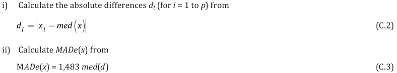
EXAMPLE: AN INFRARED THERMOMETRY ILC
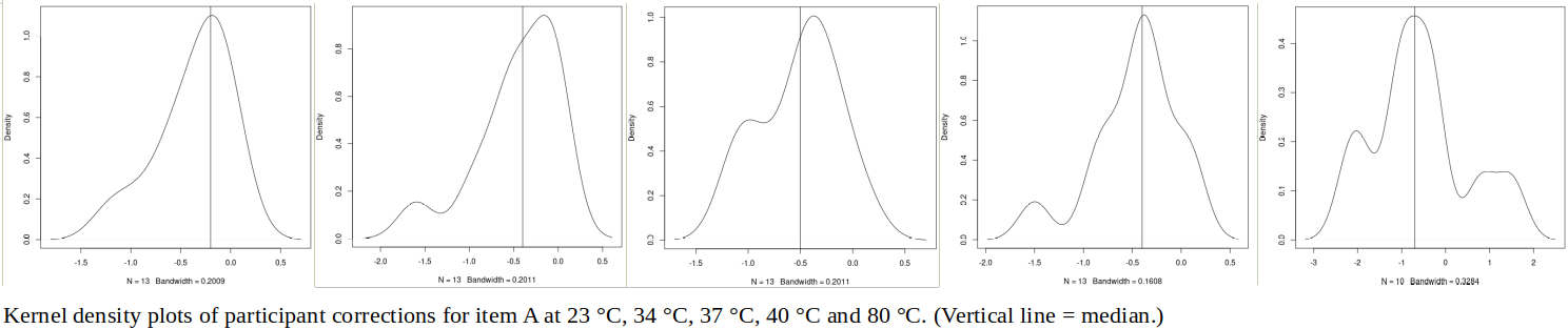
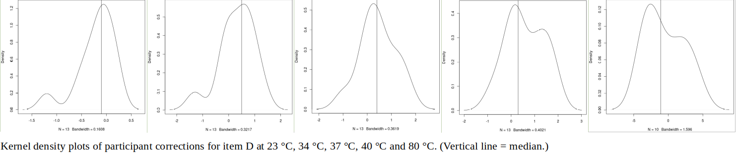
The tables below show corrections for four infrared thermometers (A to D) at five temperatures (from 23 to 80 °C), reported by a superior reference laboratory (Ref Lab) and by 13 ILC participants (P1 to P13). As recommended in 13528 clause 6.4, graphs are presented for visual review of data. (In this case, kernel density plots [13528 clause 10.3] are prepared for items A and D.) Participant results are compared to various assigned values (Ref Lab, mean, weighted mean and median), and participant performance evaluated using En scores [13528 clause 9.7]. The results and choices of RV are discussed below.
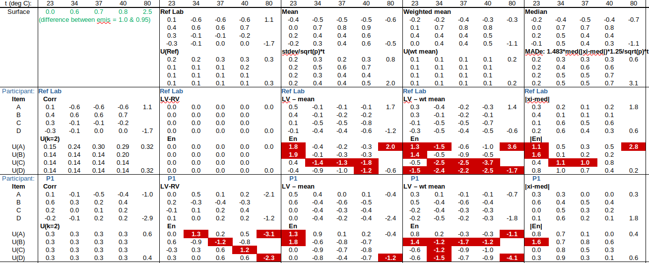
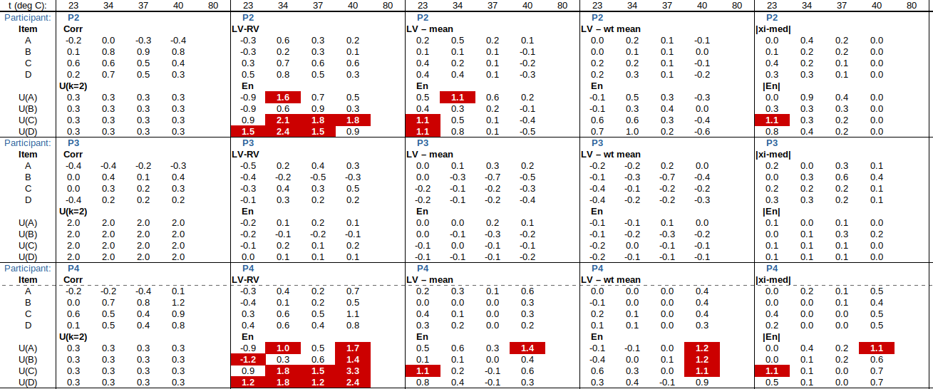
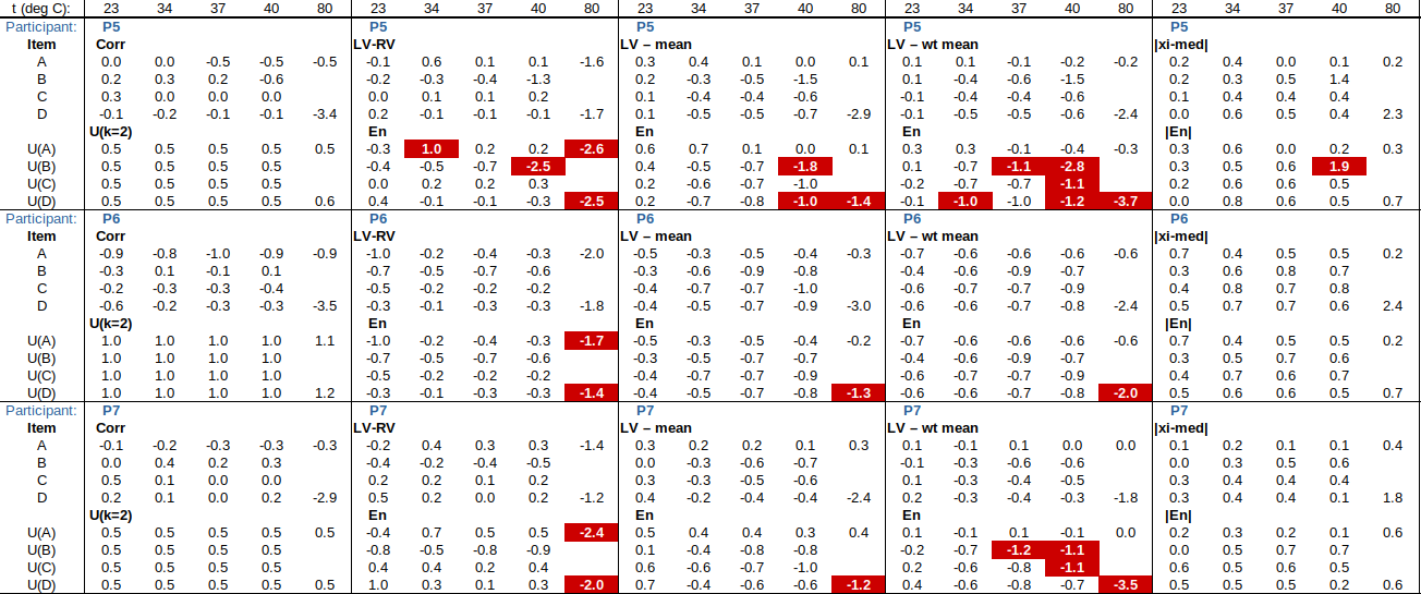
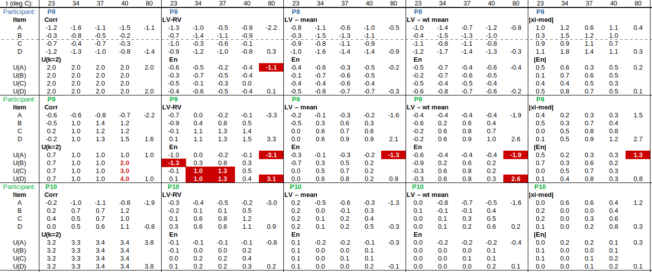
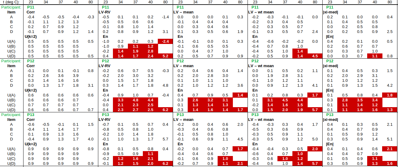
The following observations are made, regarding the above data:
∙The kernel density plots indicate that results at most temperatures are multi-modal and not symmetric, which may cause problems in data analysis, as mentioned in 13528 clause 5.3 (“Most common analysis techniques for proficiency testing assume that a set of results … will be approximately normally distributed, or at least unimodal and reasonably symmetric”). Even robust analysis techniques [13528 Annex C] assume symmetric distribution of data.
∙The spread of participant results, as represented by U(mean) or U(median), is larger than the uncertainties estimated by participants, represented by U(weighted mean), at all temperatures, but the difference is particularly large at 80 °C. This indicates that participants either neglected significant uncertainty components, or that the items drifted significantly during circulation, or both.
∙Some results of Ref Lab, particularly that for item A at 80 °C, are suspect when compared to the median of participant results. As mentioned above, even a reliable reference laboratory should be used with care.
CONCLUSION
∙Obtaining an assigned value for a PT scheme from a superior reference laboratory has the benefit of simplicity, but, as shown in a real-world example, such a Reference Value should still be checked for consistency with a consensus value calculated from participant results [13528 clause 7.8].
∙The use of participant uncertainties to estimate
∙Using the spread of participant results to estimate
∙Visual review of PT data, for example using kernel density plots, is a convenient way to obtain an overview of what may be a large and complex data set.
∙Two techniques for removing bias from a consensus value are: (i) If there are multiple participants from some laboratories, use only one result from each laboratory to contribute to
Contact the author at LMC-Solutions.co.za.
 (1)
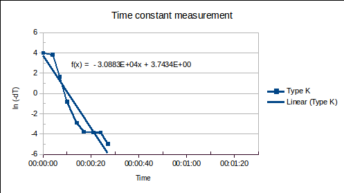
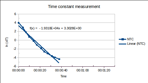
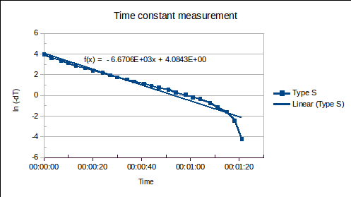
(1) is the time since the sensor was plunged into an environment of temperature
  ,
,  is the initial temperature of the sensor, and
  is the time constant.
 , of the sensor and the heat transfer coefficient,
  , from environment to sensor:
  . It may be determined by measuring
  versus
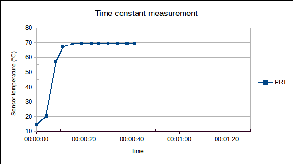
 (1a)
(1a)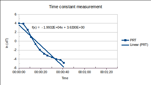
 , where
  is the number of readings.)
 .
. is the combined mass of the piston, sleeve (weight carrier) and the weights used. The uncertainty of calibration may be
  (around
  , may be measured to better than
  , in which case its uncertainty is negligible. However, if it is estimated by a
  may be
  , which is significant. The certificate typically reports
  uses conventional air and weight densities (1.2 kg.m^-3 and 8000 kg.m^-3), not the actual ones. The buoyancy correction is around
  : the additional
  for deviation from conventional air density, and its uncertainty, is often negligible (
 below 300 m altitude).
 , is unimportant for pneumatic systems. For hydraulic ones, the contribution to total weight may be
  , important to correct for, but whose uncertainty has a negligible effect.
 , has an uncertainty around
  : this is usually the dominant component of total DWT uncertainty, especially at high pressures. The pressure distortion coefficient,
  , is ~
 per MPa, i.e., the correction goes up to
  at 500 MPa. Say its uncertainty is 10% of its value, i.e., up to
  at lower pressures. The thermal expansion coefficient,
  , is ~
 per °C. So, for
  ~1 °C, the contribution to
  is around
  is ~1000 times smaller than for oil, the head correction,
  , is often negligible. The uncertainty in the head correction is typically dominated by
  , i.e.,
  and
and  are negligible. If h~0.27 m (as in the Fluke P3830 pressure balance) and
  , one of the two largest contributors. At higher pressures, the
  term dominates and U(head) becomes less important (e.g.,
  contribution to
  (sensitivity coefficient =
  )
) (sensitivity coefficient =
  )
) )
) )
) . The absolute accuracy of the balance used to weigh the dishes is not important, nor are the absolute times indicated by the watch: only the changes are of interest.
 ? We could evaluate the sensitivity of the balance [
 , or 27%. Note that this is significantly worse than the balance sensitivity of 1% of total mass gain (which would translate to 0.000 001 g/h) required in the test methods [E96 clause 6.3, 952-1 clause 6.11.4.2.2], indicating that balance sensitivity is, in this case, negligible compared to other factors causing “noise” in the mass readings. It highlights the importance of having more data points than unknowns and performing a least squares fit, as this uncertainty component would otherwise be grossly underestimated. It also shows how the standard error in the slope is far more useful than the correlation coefficient R^2, in quantifying uncertainties.
 ? (In the previous paragraph, it seems we already obtained a “complete” uncertainty for the slope. However, the fitting procedure we used assumes no uncertainty in the x-values, only uncertainty in the y-values, so we had better look at the uncertainty in the time intervals, too.) The documentary standards require time intervals to be measured to an accuracy of 1% (for example, a 24 hour interval to an accuracy of 15 minutes), so,
  [E96 clause 11.3, 952-1 clause 6.11.4.2.2]. We can see that the relative uncertainty in
  . When parameters are combined by simple multiplication or division, the relative uncertainties may be added simply in quadrature. So,
  . As
. As  is typically smaller than 0.01, it, like
  , can be neglected, so that the final relative uncertainty is
  , or 27%. In other words, U(k=2) = 1.00 g/m^2/24h * 0.27 = 0.27 g/m^2/24h.
 . If the uncertainties are quite different, the weighted mean (giving more weight to those specimens with smaller uncertainties) could be used:
  . The uncertainty of the weighted mean is
  , which also works out to be 0.16 g/m^2/24h, in the above example.
 , of a
  , on the
  at several temperatures
  , together with their uncertainties,
  , to calculate ITS-90 deviation function coefficients and propagate uncertainty, is covered in papers such as
  and to estimate
  for one fixed point temperature.
 , to that at the triple point of water (0.01 °C),
  .
. and
and  the measurement at the fixed point.
 , is constant (except for its temperature variation, considered in the uncertainty analysis, later), using
  , or just
  , will give the same resistance ratio. This applies for all resistance records mentioned below, except when noted otherwise.
 , and “resistance ratio”,
  .
. , resistances
  , or bridge ratios.)
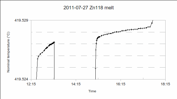
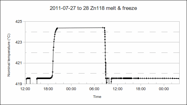
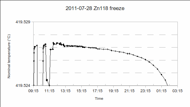
 . As the furnace temperature is several °C colder during freeze than melt, this difference in PRT readings indicates the sensitivity (if any) of the PRT to the environment outside the fixed point cell.
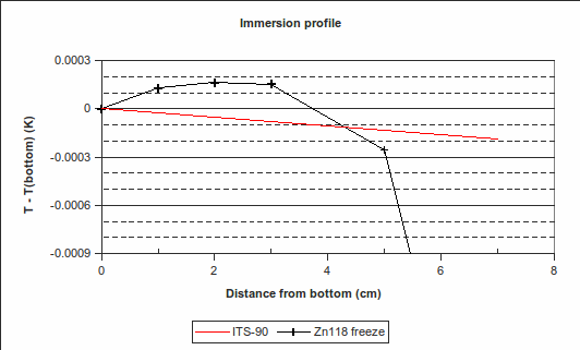
 :
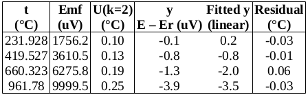
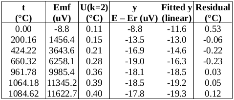
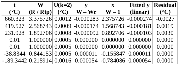
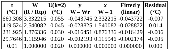
: we will use the value at the start of the freeze (the resistance equivalent to 419.527 2 °C), namely, 65.619 14 Ω.
 .
. for zinc [ITS-90 Table 2], yielding 0.000 1 °C (k=1). For the WTP cell, the residual gas pressure may be estimated by the inverting the cell and observing how much the remaining
  . Using this information, the uncertainty in the liquidus temperature may be estimated using the “overall maximum estimate” (OME) method:
  , where the cryoscopic constant
  for zinc, so that
  (k=1) [CCT-WG3 guide, equation (2.23) and Appendix B]. (The melting range following a slow freeze was previously recommended as an indicator of purity: the purer the material, the narrower the melting range. However, some significant impurities may not betray their presence by an increased melting range, so this range is only used for quality assurance purposes now, to indicate changes in the cell or furnace condition.) For the WTP cell, we have no impurity information, so we use a literature value of 0.000 05 °C (k=1.732) [CCT-WG3 guide, section 3.2]. Likewise, for the isotopic composition of the water, we use a literature value of 0.000 1 °C (k=1.732) [CCT-WG3 guide, section 3.3].
 , suggesting that the lower furnace temperature during the freeze causes the PRT to be colder than expected during that plateau. To be conservative, we will use the larger of these values, 0.001 2 °C (k=1.732), as the uncertainty due to immersion and thermal effects for zinc. For the WTP, the following immersion profile was measured:
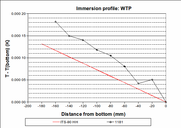
 , which is 0.000 02 °C (k=1.732) in temperature units. The effect of variation in
  (k=2) in units of bridge ratio. To find the uncertainty in
  . The maximum variation in its temperature during the measurements is estimated to be 0.2 °C (k=1.732), yielding an uncertainty in
  , or 0.000 07 °C (k=1.732).
 , propagate that to the zinc temperature by multiplying by W(Zn), then combine it with the other components relevant to the zinc point. In doing this, beware of double-counting components: Variation in
  , so is also only counted once.
 . (Actually, as the dominant component follows a rectangular distribution, we’re entitled to use k=1.65 [
 , with an uncertainty of 0.1 °C (coverage factor k=2). A resistance thermometer is used to measure the air temperature,
  , where
  is the actual vapour pressure of water and
  is the saturation vapour pressure of water at the prevailing temperature [
 , where
  is used for the irrational number 2.718… (to distinguish it from the symbol for vapour pressure), and the constants are
  and
and  [Guide to the measurement of humidity, Institute of Measurement and Control, 1996, p 53]. The Magnus formula has an uncertainty of less than 1.0 % (k=2) from -65 °C to 60 °C. We will not apply the water vapour enhancement factor to
  .
. , then manipulate the Magnus formula to obtain
  [Guide to the measurement of humidity, Institute of Measurement and Control, 1996, p 54].
 and
and  :
:

 or
or  , in other words, RH changes by approximately 6% of the value, for a change of 1 °C in dew point or air temperature. (The symbols °Cfp and °Cdp, for “degrees Celsius frostpoint” and “degrees Celsius dewpoint”, are commonly used to distinguish dew-point temperature, a measure of humidity, from air temperature.) In other words, if
  by comparison with a 1 kg weight of class
  (weight classes are described in
  of a standard weight that balances this body under “conventional” conditions, namely, ambient temperature
  = 20 °C, air density
  and standard weight density
  [D 28 section 4, p 5]. The conditions have been chosen such that mass,
  , and conventional mass,
  [R 111-1 section 5.2 and Table 1, p 11-12], or, equivalently, a relative standard uncertainty of
  , that typical deviations of weight density from the conventional
  [D 28 equation 1, p 6].
 , with the largest calibration uncertainty allowed by R 111-1 for class


 (see below for calculation)
 is
is  lower than
  : this difference is large (compared to the
  relative uncertainty goal), although the assumed weight density is not far from ideal.
 , the sensitivity coefficient of
  will be calculated using the worst-case scenario: as
  for 1 kg
  for 1 kg
  will be used. (The calculation is performed below.)
 , and, consequently, air density
  , are unusually low, because the measurements were performed at an altitude of 2400 m. The even-more-approximate formula for air density,
  [R 111-1 equation (E.3-2), p 76], yields a similar air density,
  .
.
 . Sensitivity coefficients come from R 111-1 section C.6.3.6 (p 68), with
  and
and  being converted from
  to
to  and from fractional relative humidity to %rh, respectively. (Both change by a factor of 100, though in opposite directions.) It is clear that air pressure has the largest effect on air density, followed by temperature, with the effect of relative humidity being negligible.
 [D 28 equation (9), p 8],
 is the measured difference in apparent masses.
 [D 28 equation (10), p 8] is applied, because the air density differs from
  by more than 10 % [R 111-1 section 10.2.1, p 18].
 , we’ll need the sensitivity coefficients
  ,
,  and
and  .
. , where
  (the uncertainty of the weighing process and the balance, combined) and
  , in the notation of R 111-1 section C.6, p 66-70.
 .
. .
.

 ,
, is the air density during the last calibration of the reference weight.
 ,
, 
 +
+  , with the terms in
  and
and  dominating over the term in
  contains the uncertainty of the weighing process,
  , which is an ESDM calculated as 0.01 mg, the sensitivity of the balance,
  , and the display resolution of the balance,
  . (Eccentric loading of the balance is included in
  , so that
  .
. . So, we have achieved our goal of a relative standard uncertainty smaller than