When we calibrate a temperature sensor by comparing it to a reference standard thermometer, we try to keep the comparison medium (hereafter called the “environment”) stable in temperature during the period of comparison. (By “stable”, we mean that the fluctuation in the temperature of the environment is small relative to the desired uncertainty of calibration.) But, what happens if the environment temperature does vary significantly during the process of recording reference standard and unit under test (UUT) readings? This article discusses the comparison of temperature sensors with different response times in an unstable environment. It reports measurements of time constants of several types of sensors, and their comparison in a stirred water bath with large temperature fluctuations (on-off, rather than PID, control). The appropriate choice for the uncertainty contribution arising from temperature instability is then justified by an analysis of the measured data.

Temperature sensors do not respond instantaneously to changes in the temperature of the environment they are intended to measure. If a sensor is plunged into an environment, the rate at which the sensor temperature approaches that of the environment is described by Newton’s law of cooling, which leads to the equation
     (1)
[J. V. Nicholas, D. R. White, Traceable Temperatures, 2nd ed, 2001, p 141], where is the time since the sensor was plunged into an environment of temperature ,  is the initial temperature of the sensor, and  is the time constant.
is the time the sensor takes to undergo ~63% of the total change in temperature. It is a function of the heat capacity, , of the sensor and the heat transfer coefficient, , from environment to sensor: . It may be determined by measuring  versus  and modelling the data using equation (1).
(Note that, although the heat capacity is constant for a particular sensor, the heat transfer coefficient varies according to the environment, so that the time constant of a sensor in still air may be tens of times longer than the time constant of the same sensor in stirred water.)

Infrared radiation (non-contact) thermometers typically respond very quickly (response time < 1 s), but this article focuses on immersion probes, which are in physical contact with the environment. The sensors studied were a mineral-insulated, metal-sheathed (MIMS) platinum resistance thermometer (PRT) and type K thermocouple, an epoxy-coated NTC thermistor and a ceramic-sheathed type S thermocouple, with a brief mention of a solid-stem mercury-in-glass thermometer.

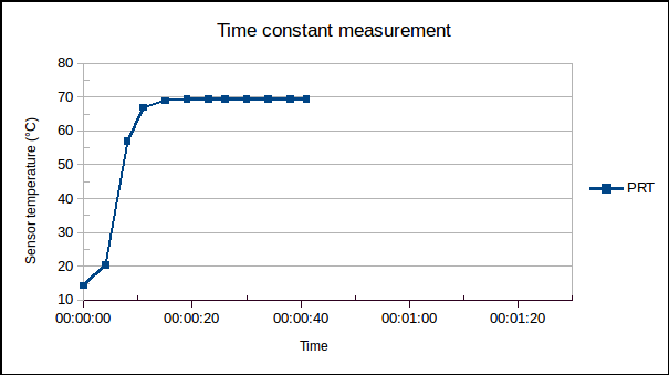
First, the time constants were determined by plunging the sensors from an ambient temperature of 15 °C into a stirred water bath controlled at 70 °C. The temperature readings of the PRT are plotted vs time, below:

Equation (1) was manipulated to allow a straight line to be fitted:
    (1a)
The linearised data and fitted straight lines are plotted, below:

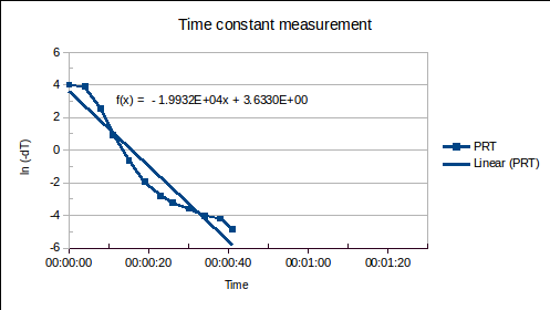
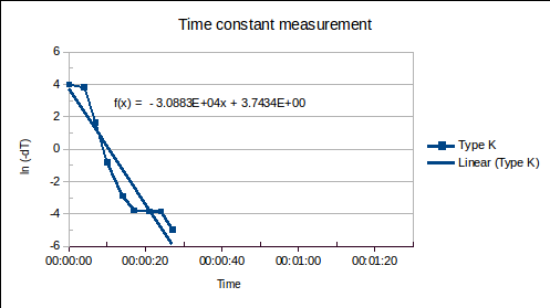
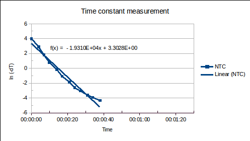
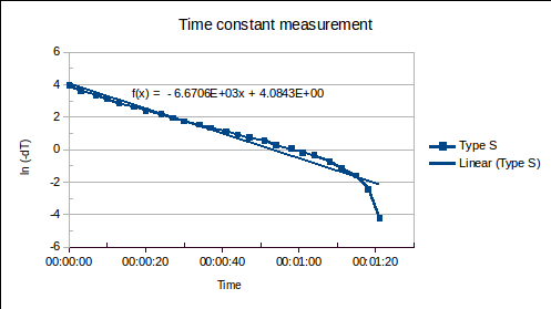
The following time constants were found. (Time is in units of days in the straight lines fitted to the data above, therefore, so is . It is converted to seconds in the table below.)

Sensor	t0 (seconds)
6.4 mm diameter MIMS PRT	4.3
6 mm diameter MIMS type K thermocouple	2.8
Epoxy-coated NTC thermistor	4.5
6.7 mm diameter ceramic-sheathed type S thermocouple	13.0

The following points were noted:
1. The multimeter used to measure both RTD resistances and thermocouple voltages was set to a slow measurement rate (signal integration over 5 power line cycles or 0.1 s), which may have affected the measured values somewhat.
2. The longer time constant of the ceramic-sheathed type S thermocouple is expected, as the alumina ceramic is less thermally conductive than a metal sheath, there is an air gap between this sheath and the twin-bore alumina insulator holding the thermocouple wires, and these wires are probably thicker (0.4 mm) than those in, for example, the MIMS type K thermocouple. Such a high-temperature laboratory standard thermocouple construction is expected to exhibit the longest time constant of the sensors typically calibrated in a temperature calibration lab.
3. The results show fair agreement with previous measurements of  = 5.2 s and 2.9 s, for a heavier 6.4 mm MIMS PRT and a 6.25 mm solid-stem mercury-in-glass thermometer, respectively.

The water bath controller was then adjusted from PID to on-off control, resulting in a control cycle of ±0.5 °C with a period of ~140 s. The following measurements were recorded from the four sensors (vertically offset on the graph, for greater clarity):

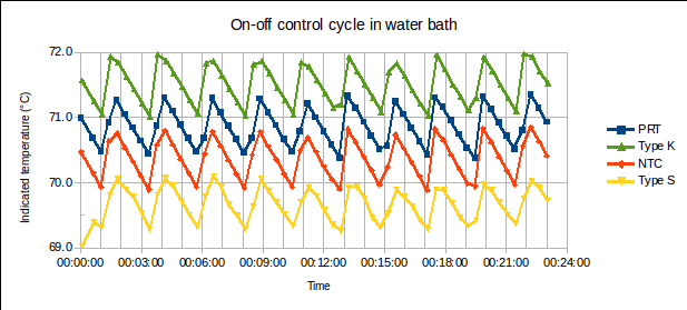
From these 58 measurements, over 10 control cycles (23 minutes), the following results were obtained. (Fluctuation in the absolute temperature reading of each sensor is labelled “abs” in the table below. The PRT was considered as the reference standard: the mean deviations of the other sensors relative to the PRT, labelled “dev” below, would be the results reported in their calibration certificates. The experimental standard deviation of the mean, or ESDM, is , where is the number of readings.)

	PRT	Type K		NTC		Type S
	abs	abs	dev	abs	dev	abs	dev
Mean_all (°C):			0.65		-0.50		-1.19
Std dev (°C):	0.29	0.31	0.12	0.30	0.07	0.25	0.11
ESDM (°C):	0.04	0.04	0.02	0.04	0.01	0.03	0.01

A sample of six measurements was taken from these 58, representing a data set that might be captured during a typical calibration:

	PRT	Type K		NTC		Type S
	abs	abs	dev	abs	dev	abs	dev
Mean_sample (°C):			0.68		-0.48		-1.15
Std dev (°C):			0.15		0.10		0.04
ESDM (°C):			0.06		0.04		0.02
Mean_smp – mean_all (°C):			0.03		0.02		0.04

The following points were noted:
1. The standard deviations of the “absolute” readings are smaller for those sensors with longer time constants (particularly, the type S thermocouple). This is as expected: the sensor response to a sinusoidally varying input is attenuated as the time constant becomes larger relative to the period of oscillation. (In other words, a sensor with more thermal inertia will exhibit less peak-to-peak variation in reading, the faster the control cycle.)
2. The mean of the 10% sample agrees with the mean of all 58 measurements (considered representative of the population) within approximately the ESDM of the sampled deviations: this level of agreement between the sample mean and the population mean suggests that the ESDM of the deviations is the appropriate value to use for the uncertainty component “temperature instability”.
3. The standard deviation of the absolute readings (~0.3 °C, as expected for a control cycle of ±0.5 °C) is about three times larger than the standard deviation of the deviations. Using the standard deviation of the absolute readings of the UUT (or, even more so, the standard deviations of the absolute readings of both reference standard and UUT) as the value(s) for “temperature instability” in the uncertainty budget would overestimate this contribution to the total uncertainty of calibration.

The period of oscillation of the environment’s temperature (~140 s) was long relative to the time constants of the sensors (3 to 13 s). In such a situation, a lag error of up to ~[(13 – 3) s * 0.01 °C/s] = 0.1 °C might exist between the slowest and fastest sensors evaluated, during a part of the control cycle when the environment temperature was monotonically falling or rising. (The rate of cooling is ~0.01 °C/s in the above data, and the rate of heating somewhat faster.) However, provided that the recorded data originate from varying points along the control cycle (not always when the reference standard is rising, for example, but equally often when it is rising and when it is falling), the fluctuation in the difference between reference standard and UUT provides an adequate estimation of the uncertainty contributed by the unstable environment. (The slow sensor will be colder than the fast sensor while the environment is heating, and hotter than the fast one while the environment is cooling: using enough measurements, taken randomly during several control cycles, the average of the differences between the slow and fast sensor will cancel out the effect of differing response time.)

Contact the author at LMC-Solutions.co.za.