ABSTRACT
This publication follows “Interlaboratory comparisons (Proficiency Testing) among calibration laboratories – how to choose the assigned value (Reference Value)” of October 2025, describing additional techniques for visualizing and interpreting results. Participants’ reported probability distributions are combined for visual review, Cox’s Largest Consistent Subset approach is applied to remove outliers, and the recommendations in this and the previous paper are applied to a small Thermometry ILC with four participants.
VISUAL REVIEW OF DATA
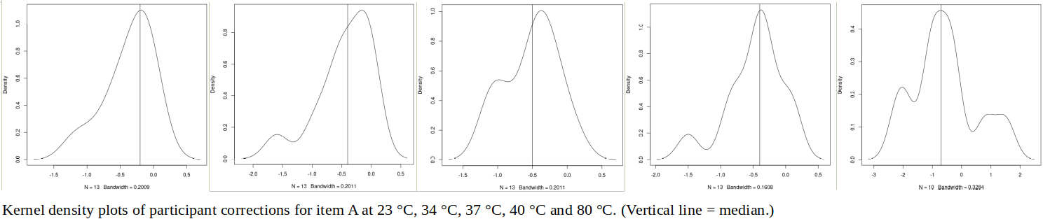
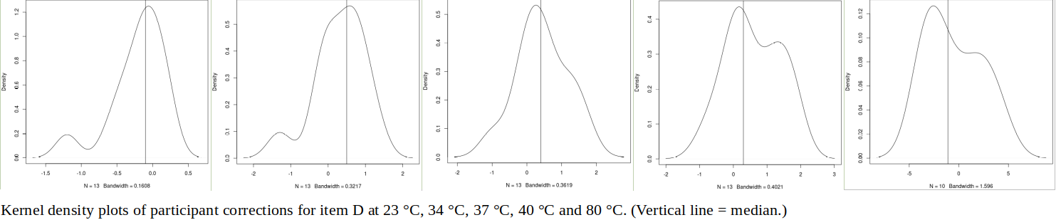
First, we continue to discuss the infrared thermometry ILC involving Ref Lab and 13 participants, from the previous paper: The kernel density plots, that were used to examine the data for items A and D, combine normal distributions with equal standard deviations (widths) around each participant’s result. (Plots were generated using the density() function in the R programming language.) What would the plots look like, if the widths were derived from the participants’ estimated uncertainties (which vary by an order of magnitude)? And, what would be the effect of including Ref Lab in the combination (convolution) of normal distributions?
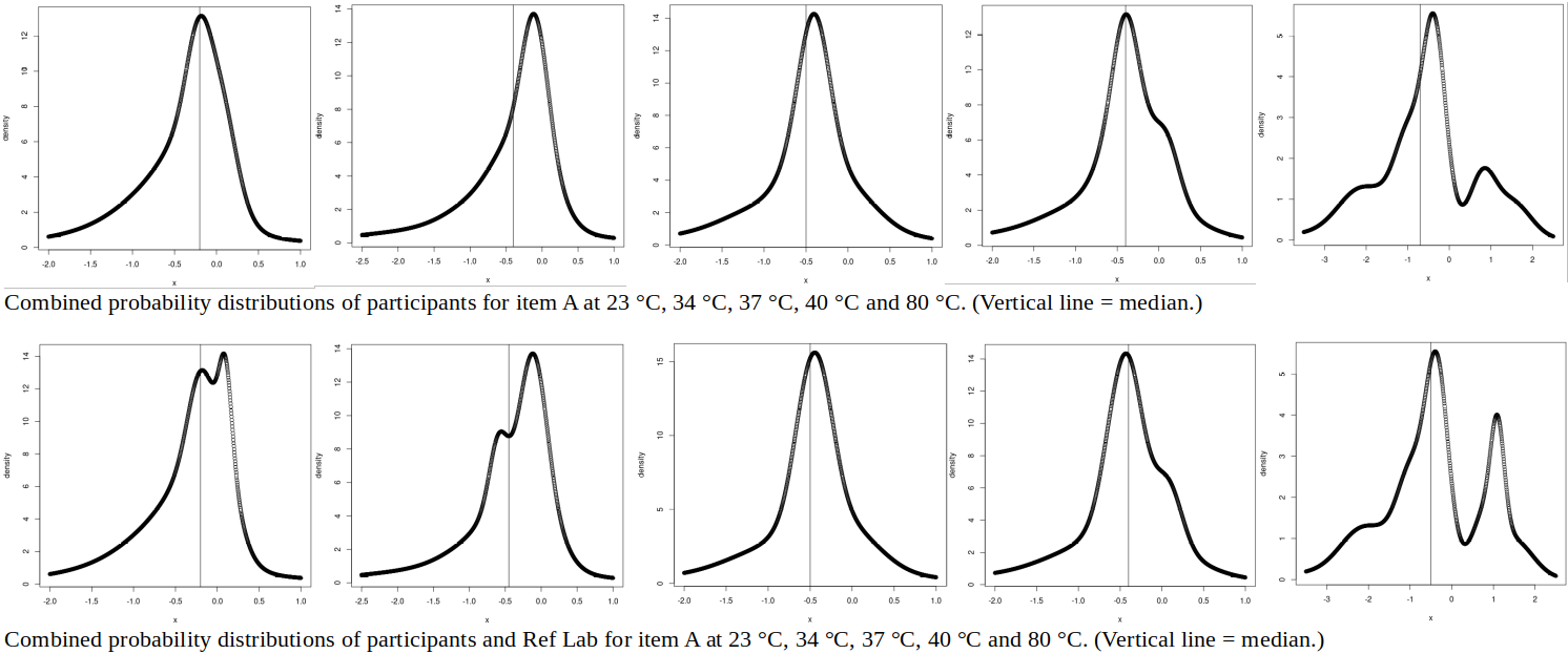
For item A, using the participants’ uncertainties (second row of graphs above) tends to “smear out” the secondary modes (lower peaks) observed in the kernel density plots, suggesting that results in these areas have larger estimated uncertainties. (The effect is similar to enlarging the bandwidth of the kernel density plot.) Including the Ref Lab results in the combined distributions (third row of graphs) adds or heightens a peak in the 23, 34 and 80 °C data. As Ref Lab has the smallest uncertainties, it produces sharp, high peaks. (This is similar to how the weighted mean is dominated by the results with the smallest uncertainties.)
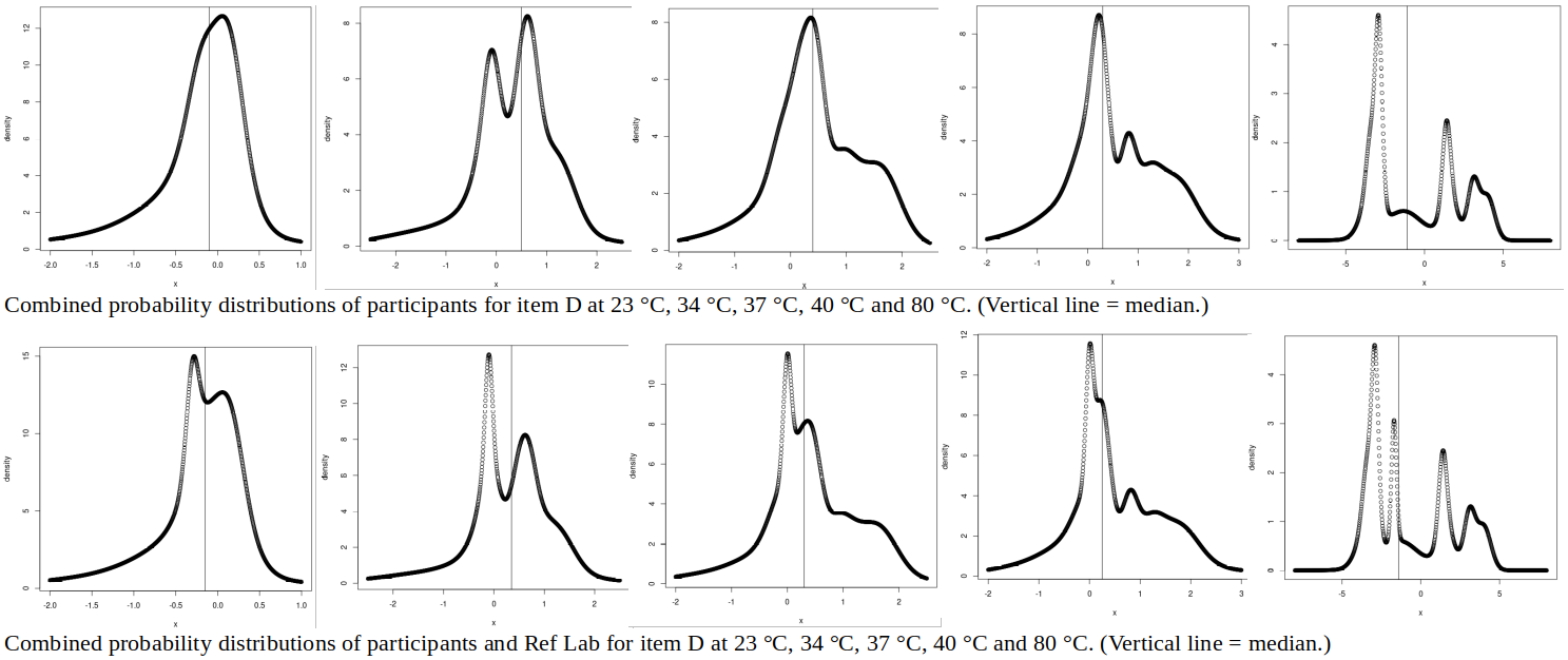
For item D, using the participants’ uncertainties removes the secondary peak for 23 °C, splits the main peak for 34 °C into two, and reduces the secondary peak for 40 °C.
For 80 °C, two peaks become three: -3 K (participants P1, P5, P6, P7), +1.5 K (P9, P11) and +3 K (P12, P13). It is interesting to observe that, if their uncertainties are small, just two participants (out of p = 10) can create a significant peak. Ref Lab’s result at 80 °C lies around halfway between the -3 K and +1.5 K peaks: does this suggest a difference in method between P1-P5-P6-P7 and P9-P11, Ref Lab applying a measurement technique halfway between these two populations? A similar split (P1-P2-P3-P5-P6-P7 vs P9-P10-P11) may be present at 40 °C, but the differences are smaller and therefore less distinct.
(It should be noted that Ref Lab and participants P1 to P8 used blackbody targets with emissivity ≈ 1.00, while P9 to P13 used flat plates with ε ≈ 0.95. The latter results are corrected to ε ≈ 1.00 (corrections ~ 0.7 K around 37 °C and 2.5 K at 80 °C), but perhaps some emissivity-related effects remain.)
A general observation, regarding the convolution of reported results (with widely differing uncertainties) vs the use of a kernel density plot (with equal bandwidth for all results): In practice, calibration laboratories using similar measurement standards and equipment (and therefore having similar measurement capabilities in reality) may report very different uncertainties, because, for example, some accredited CMCs are conservative and others are not. For this reason, it is suggested that reported uncertainties are of little value in visualizing the distribution of results, and a kernel density plot (with equal bandwidth for all results) is recommended.
LARGEST CONSISTENT SUBSET OF RESULTS
The above distributions of results are mostly multi-modal (having several local maxima) and asymmetric. Would the removal of “inconsistent” results improve the situation? (Our ideal combined distribution would be symmetric, with only one peak.) [Cox, “The evaluation of key comparison data: determining the largest consistent subset”, 2005] proposes a chi-squared test for consistency between the Weighted Mean (assigned value, y) and the participants’ results, x_i, with the “worst” results (largest contributors to chi-squared) being removed one-by-one, until the observed chi-squared value “passes” and we are left with the “Largest Consistent Subset” (or, LCS):
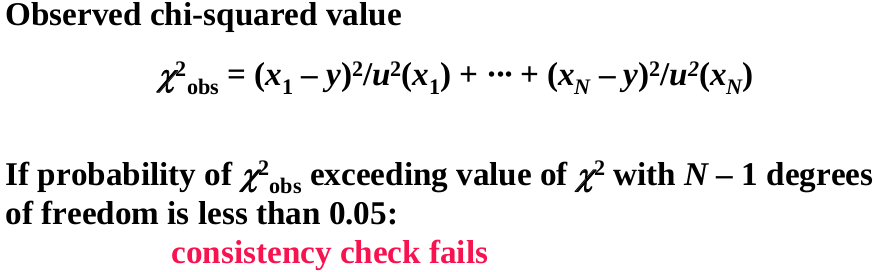
(The threshold value of Χ^2 may be calculated using the spreadsheet function CHISQ.INV.RT(0.05,N-1), where N = number of participants contributing to RV, or the Largest Consistent Subset may be directly determined using the LCS() function in the metRology library of the R programming language.)
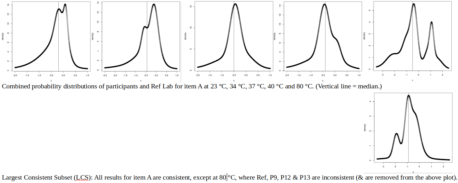
For item A, only the 80 °C results are inconsistent (according to Cox’s criterion), and the removal of inconsistent results to find the “Largest Consistent Subset” (second row of graphs above) does not, unfortunately, create a unimodal or symmetric plot.
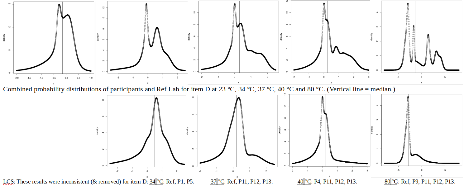
For item D, all but the 23 °C results are inconsistent. Removing inconsistent results does improve the appearance of the combined probability distributions, though some asymmetry remains.
The LCS approach to finding an assigned value (or Key Comparison Reference Value, KCRV, for a Key Comparison between National Metrology Institutes) is intended to produce the best estimate of the SI value of the measurand [Cox, “The evaluation of key comparison data: determining the largest consistent subset”, Metrologia 44 (2007) 187–200]. This is seldom the goal for an interlaboratory comparison (ILC) between commercial calibration laboratories, where each participant simply aims to demonstrate his equivalence to a “credible” Reference Value. Bearing this in mind, and considering that the number of participants in a typical calibration ILC is small (7 or less, according to [EA-4/21 INF: 2018, “Guidelines for the assessment of the appropriateness of small interlaboratory comparison within the process of laboratory accreditation”]), the removal of participants from RV using a chi-squared test is not always reasonable: the reported uncertainties used to calculate chi-squared may be unrealistic, and the resultant number of results contributing to RV may be too small for statistical confidence. Instead, it is suggested that commercial calibration laboratories arranging a small ILC use a “consensus value from participant results” [ISO 13528:2015 section 7.7], using “a subset of participants determined to be reliable, by some pre-defined criteria … on the basis of prior performance” [13528 clause 7.7.1.1], with this “prior performance” being their reputation in the relevant field. An example of such a small ILC is presented below.
EXAMPLE: A SMALL INFRARED THERMOMETRY ILC
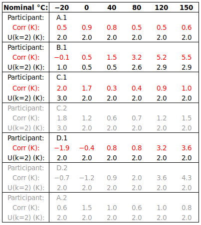
In this example, one infrared thermometer was calibrated from -20 to 150 °C. The pilot laboratory invited the other three laboratories to participate based on their reputation for competence in the field, so that all four laboratories might contribute to RV. Viewing conditions were specified (100 mm from a 50 mm diameter target, or 300 mm from a 150 mm target, etc), so that differing Size-of-Source Effect would not render the results incomparable. Three laboratories submitted multiple result sets (measured by different metrologists), but selected one set to contribute to RV, as required by the protocol. The results are presented below, in the sequence in which they were measured, with secondary results from relevant laboratories being identified as “x.2″:
VISUAL REVIEW OF DATA
The results are plotted, relative to the mean correction, below:
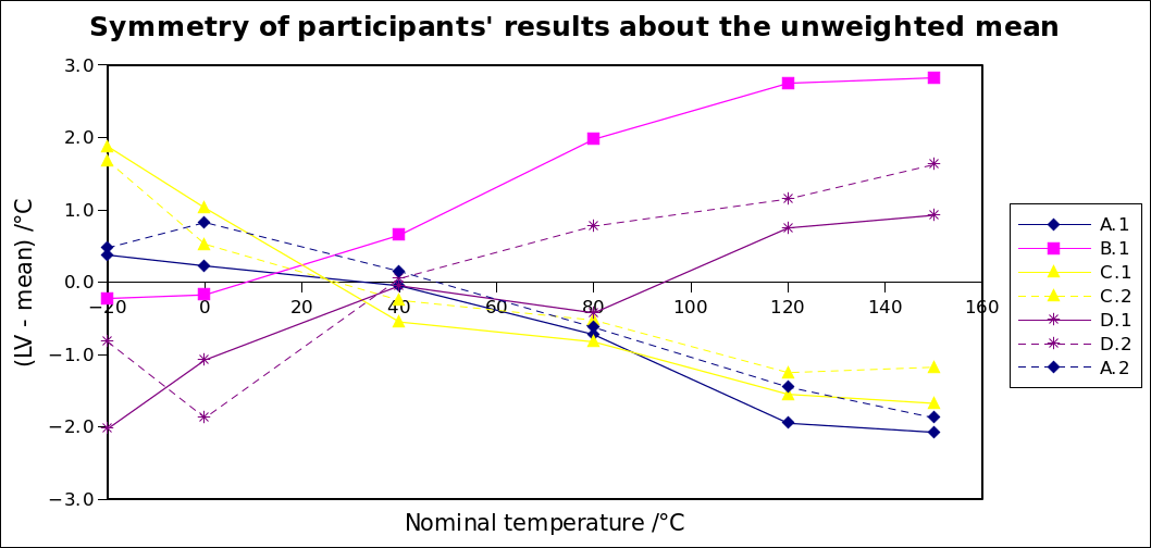
The expected tight grouping of results within a laboratory may be clearly seen in laboratories A, C and D. Good agreement between initial and final measurements at laboratory A (results A.1 and A.2) indicates that the thermometer was stable during the one-month circulation.
Kernel density plots of the four “primary” results (chosen for inclusion in RV) are shown below:
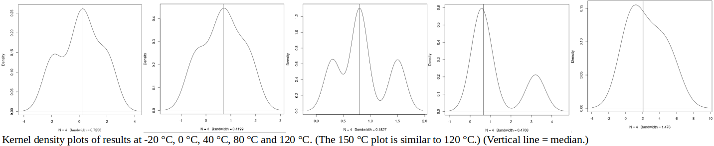
It is observed that these kernel density plots allow for better visual review of the data than does the graph of results relative to the mean. (There is significant asymmetry in the 80 °C and 120 °C results, which was not obvious in the graph relative to the mean.)
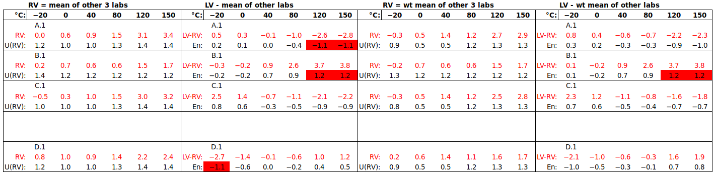
a) U(RV) FROM PARTICIPANT UNCERTAINTIES
Two Reference Values are considered, the mean and the weighted mean. For each laboratory, RV is calculated from the results of the other three, to avoid the laboratory being “compared to itself”. The uncertainty of the mean is estimated from reported participant uncertainties by 

As seen below, either value of U(RV) is smaller than U(LV), for all but participant B.1 at lower temperatures, so tests the capabilities of laboratories A, C and D fairly rigorously. It does not, however, meet the criterion for uncertainty of the assigned value u(x_pt), relative to the “performance evaluation criterion” σ_pt, suggested in ISO 13528 clause 9.2.1, namely
![]()
(If this criterion is met, then the uncertainty of the assigned value may be considered to be negligible.)
As mentioned above, the uncertainties reported by commercial calibration laboratories in ILCs differ widely, often without any technical justification. For this reason, it is recommended to use the unweighted mean as the Reference Value. However, as the goal of the ILC is to demonstrate equivalence between participants within their reported uncertainties, U(RV) is estimated from these reported uncertainties, not from the observed spread of results.
b) U(RV) FROM SPREAD OF PARTICIPANT RESULTS
The median is often used as a robust Reference Value for large ILCs, with its uncertainty being estimated from the spread of results via the scaled median absolute deviation (MADe). Is the median an appropriate Reference Value for a small ILC?
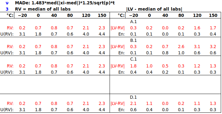
(Note: In the above table, the median and its uncertainty are calculated using all four results, i.e., not excluding the participant’s own result.)
It is observed that, while the median may be a reasonable Reference Value for such an ILC, the uncertainty of the median, being derived from the spread of the participants’ results, is not suitable for the task of demonstrating equivalence within reported uncertainties. To achieve this goal, U(RV) should be derived from the reported uncertainties. Also, U(median) is often larger than U(LV), so does not test participants’ capabilities rigorously.
CONCLUSION
∙Kernel density plots are recommended for visual review of data (the first step in analysis of ILC results).
∙The ILC report should present participants’ results in the order in which they were measured, so that readers may themselves look for artefact drift.
∙If a laboratory submits multiple result sets, it should choose one set to contribute to a consensus Reference Value, before having sight of other participants’ results.
∙The ILC report should indicate which result sets are from the same laboratory, so that readers may interpret data clustering correctly.
∙For small ILCs, each participant should be evaluated against a Reference Value derived from other participants’ results (to avoid bias).
∙To promote the credibility of RV, a subset of participants may be pre-selected to contribute to it, on the basis of “prior performance” (reputation in the field).
∙If a consensus Reference Value is to be used, the mean is recommended, rather than the weighted mean, as reported uncertainties often vary widely, without technical justification.
∙The uncertainty of a consensus Reference Value, U(RV), should be determined from participants’ reported uncertainties, rather than from the spread of results, to achieve the goal of demonstrating equivalence within reported uncertainties.
∙Technical assessors should ask: Is RV credible? (Is it composed of reputable labs?) Does it omit the laboratory being tested, especially if the number of participants is small? Is U(RV) < U(LV), in order to test the participant’s capability rigorously?
Contact the author at LMC-Solutions.co.za.