ABSTRACT
In preceding publications, the accuracy of interpolation using reference functions for temperature sensors (thermocouples and platinum resistance thermometers (PRTs)), as well as a crude approach to interpolation uncertainty in the absence of any knowledge of the interpolating function, have been discussed. This article discusses how to fit curves to PRT calibration results using the linear least squares technique (implemented using matrix functions in Microsoft Excel or Libreoffice Calc), both directly to the measured data and to deviations from a reference function. (An overview of the fitting method may be found in [Numerical Recipes in Fortran 77, Chapter 15. Modeling of data].)

INTRODUCTION

In the preceding articles, we saw that
(i) industrial PRT calibration results could be interpolated “piece-wise” (between any two calibration points a few hundred degrees Celsius apart) to an accuracy of around 0.05 °C, when expressed as deviations from the Callendar-van Dusen reference functions, and,
(ii) without any knowledge of the accuracy of the interpolating function, the accuracy of interpolated values could be grossly estimated as 0.15 to 0.5 °C (for the above-mentioned spacing between calibration points).
While the latter approach can be applied generically to almost any calibration data, it has the drawback that the uncertainty of interpolated values is unrealistically large when working close to a calibration point. In the present article, the most accurate approach to the problem will be implemented, namely, to fit a curve to the complete set of calibration results. Firstly, a Callendar equation will be fitted directly to the measured data, and, secondly, a quadratic polynomial will be fitted to the deviations of the measured data from the ITS-90 PRT reference function. As the ITS-90 reference function deals with most PRT non-linearity, it is expected that the latter approach will produce the more accurate interpolation.

THE MODEL EQUATION

The Callendar equation, applicable above 0 °C, is: Rt = R0∙(1 + A∙t + B∙t^2), where Rt is the resistance (in Ω) at temperature t (in °C) and R0 is the resistance (in Ω) at the ice point (0.00 °C). Rearranging the equation, A∙t + B∙t^2 = Rt/R0 – 1, indicating that the independent variable x = t and the dependent variable y = Rt/R0 – 1.
(As the sensitivity. d(Rt/R0)/dt, will be required to convert uncertainties from temperature units, we also note that d(Rt/R0)/dt = A + 2∙B∙t. We will use the coefficients from IEC 60751, namely, A = 3.9083e-3 and B = -5.775e-7, to calculate sensitivities below.)

The measured data are as follows:

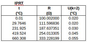
To find R0 from R(0.01 °C): R0 = R(0.01 °C) + (0.00 °C – 0.01 °C) ∙ 0.391 Ω/°C. Uncertainties are converted to the same units as y. (The 1st data point is used to determine R0, so only the four subsequent data points are used in the fit.)

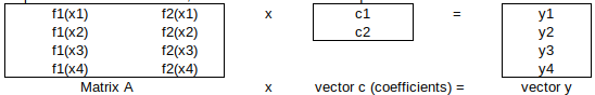
The general model equation is c1∙f1(x) + c2∙f2(x) + … = y. For the Callendar equation, c1 = A, f1(x) = x, c2 = B and f2(x) = x^2.
The four data points lead to four simultaneous equations, namely:
c1∙f1(x1) + c2∙f2(x1) = y1
c1∙f1(x2) + c2∙f2(x2) = y2
c1∙f1(x3) + c2∙f2(x3) = y3
c1∙f1(x4) + c2∙f2(x4) = y4
Expressed in matrix notation, they are:

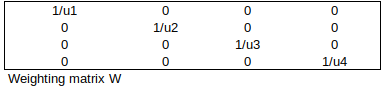
WEIGHTING FACTORS

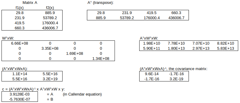
Now, apply the weighting factors 1/ui to each equation (smaller std uncertainty => larger weight). The weighted simultaneous equations, expressed in matrix notation, are: W x A x c = W x y.

THE SOLUTION – NORMAL EQUATIONS

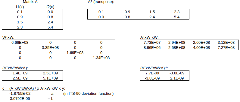
The optimal (least squares) solution to this over-determined system is obtained by left-multiplying by the matrix transpose (WA)T = ATxWT, to obtain the normal equations:

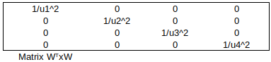
Matrix WTxW simply contains 1/variance at each calibration point:


Then, to find the fitted y-value for any value of x:


Finally, expanded uncertainty of y = 2*√variance(y): this is called the “propagated uncertainty” of y at x.

The numerical implementation of this “linear least squares” curve-fitting technique follows, using the Excel or Calc matrix functions TRANSPOSE(), MMULT() and MINVERSE():

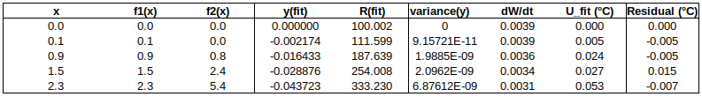
Now to check the fitted curve against the measured data (residual = measured – fitted):

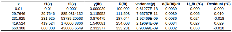
Are the residuals small enough, or, does the model fit the data well enough, relative to the uncertainties?: The chi-squared statistic, chi^2 = [(residual_1/u1)^2 + (residual_2/u2)^2 + …], will tell us:

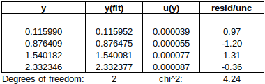
Chi-squared is larger than the degrees of freedom (= number of data points – number of fitted parameters = 4-2), so either the uncertainties are underestimated, or the model does not represent the data well (relative to the uncertainties). If chi^2 ≲ d.o.f., then the fit is “good enough”. (This is only strictly true if the uncertainties at different points are uncorrelated, but we will assume that this is the case.)

DEVIATION FROM ITS-90 REFERENCE FUNCTION

Perhaps direct fitting to the Callendar equation is not good enough, at this level of uncertainty. Let’s try deviations from the ITS-90 reference function – the reference function should take care of much of the PRT’s non-linearity, leaving us with smoother data to fit.

For the range 0 to 660 °C, the ITS-90 document gives the deviation function as: W-Wr = a∙(W-1) + b∙(W-1)^2 + c∙(W-1)^3, where W = Rt/Rtp and Wr is the value of the reference function.
It is good practice in curve fitting to use as few coefficients as will adequately fit the data, so we will try two, a and b.


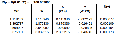
Now to check the fitted curve against the measured data (residual = measured – fitted):

It can be seen that this fit is better than the previous one. (Residuals are around half the size.)

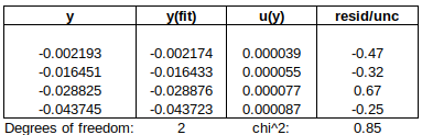
Chi-squared is smaller than the degrees of freedom, indicating that the curve fits the data well, within the uncertainties.

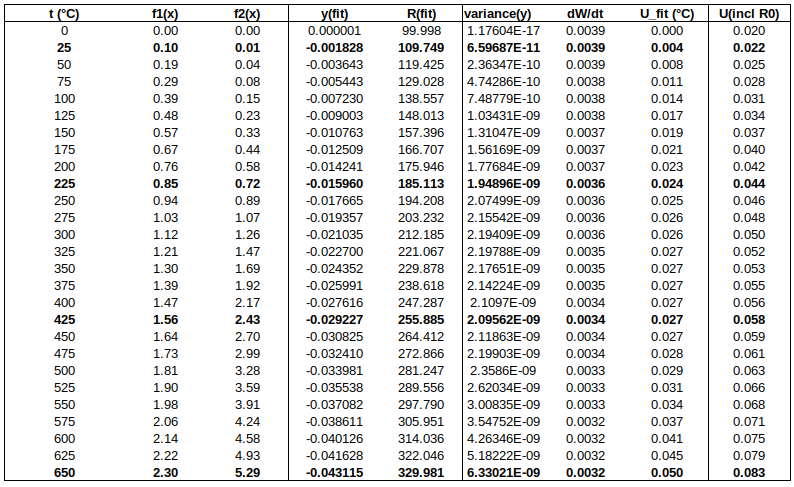
Below is a table of fitted values. Because of the structure of the ITS-90 functions, the uncertainty of the curve is zero at the water triple point (WTP, 0.01 °C). The uncertainty at WTP is added to the uncertainty of the curve, in the rightmost column.

CONCLUSIONS

∙Both curves, fitted directly to measured PRT data, and to deviations from a reference function, represent the behaviour of the UUT better than do the individual data points. (The curves take into account all the data points, thereby potentially “smoothing out” random errors in measurement.)
∙The ITS-90 deviation function fits the data better, as is expected when using a good reference function.
∙When weighted least squares fitting is performed, the covariance matrix provides a statistically justified manner of propagating uncertainty to intermediate points, which results in small uncertainties. (To be strictly correct, we should have considered possible correlation between data points, but, as long as the dominant uncertainty component(s) are uncorrelated, our approach is reasonable.)

(Contact the author at LMC-Solutions.co.za.)